Gaussian Process Practice (2) Kernels

• Gaussian Process 연습입니다.
• scikit-learn을 비롯한 예제를 재구성하여 연습합니다.
• 여러 커널의 특징을 알아보고 사용처를 알아봅니다.

1. Data Preparation

scikit-learn: Gaussian Process Regression: basic introductory example

1.1. example data

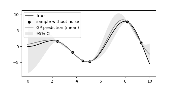
• 지난 글과 같은 예제를 사용합니다.
• 오늘은 어제보다는 색을 많이 사용할 겁니다. 참값과 Gaussian Process 결과를 무채색으로 표현합니다.
• 관측값은 참값이라고 합시다.

  %matplotlib inline
  
  import matplotlib.pyplot as plt
  import numpy as np
  from sklearn.gaussian_process import GaussianProcessRegressor
  from sklearn.gaussian_process.kernels import RBF
  
  # Random Number Generation
  rng = np.random.RandomState(1)
  
  # Gaussian Process Regression
  kernel = 1*RBF(length_scale=1.0, length_scale_bounds=(1e-2, 1e2))
  gpr = GaussianProcessRegressor(kernel, n_restarts_optimizer=9, random_state=0)
  gpr.fit(X_train, y_train)
  
  # prediction
  y_pred_mean, y_pred_std = gpr.predict(X, return_std=True)
  
  # visualization
  fig, ax = plt.subplots(figsize=(6, 3))
  ax.plot(X, y, c="k", label="true")
  ax.scatter(X_train, y_train, fc="k", label="sample without noise")
  
  ax.plot(X.ravel(), y_pred_mean, c="0.5", label="GP prediction (mean)")
  ax.fill_between(X.ravel(), y_pred_mean-1.96*y_pred_std, y_pred_mean+1.96*y_pred_std, alpha=0.5, fc="lightgray", label="95% CI")
  ax.legend(loc="upper left")

  
  

1.2. sample 추출

scikit-learn: Illustration of prior and posterior Gaussian process for different kernels

• 신뢰구간에는 다양한 가능성이 내포되어 있습니다.

• 이들 중 일부를 골라 추출할 수 있습니다.

• 5개를 골라 Gaussian Process Regression 위에 얹어봅니다.

  # sampling
  n_samples=5
  y_samples = gpr.sample_y(X, n_samples)
  
  # prediction
  y_pred_mean, y_pred_std = gpr.predict(X, return_std=True)
  
  # visualization
  fig, ax = plt.subplots(figsize=(6, 3))
  ax.plot(X, y, c="k", label="true")
  ax.scatter(X_train, y_train, fc="k", label="sample without noise")
  
  ax.plot(X.ravel(), y_pred_mean, c="0.5", label="GP prediction (mean)")
  ax.fill_between(X.ravel(), y_pred_mean-1.96*y_pred_std, y_pred_mean+1.96*y_pred_std, alpha=0.5, fc="lightgray", label="95% CI")
  
  for y_sample in y_samples.T:
      ax.plot(X.ravel(), y_sample, lw=1, ls=":", label="GP prediction (mean)")

  
  

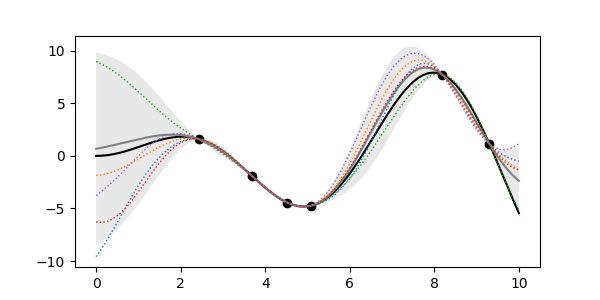
• 대부분 신뢰구간 안에 들어와 있지만 일부는 신뢰구간 밖으로도 나가 있습니다.

• 정상입니다.

1.3. posterior vs prior

• 지금 그린 그림은 evidence가 반영된 결과, 즉 posterior(사후확률)입니다.

• 학습을 시키지 않은 채 예측을 하고 sample curve를 뽑을 수도 있습니다.

• evidence가 반영되기 전의 prior(사전확률)입니다.

  # prior
  kernel = 1*RBF(length_scale=1.0, length_scale_bounds=(1e-2, 1e2))
  gpr = GaussianProcessRegressor(kernel, n_restarts_optimizer=9, random_state=0)
  
  # sampling
  y_samples = gpr.sample_y(X, n_samples)

  
  

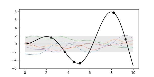
• 관측값이 반영되어 있지 않기 때문에 데이터와는 무관한 모습입니다.

• 그러나 곡선의 모양에는 우리가 선택한 RBF 커널이 드러나 있습니다.

• 학습에 커널이 반영되는만큼 데이터의 모습을 반영해 커널을 선정해야 합니다.

• scikit-learn이 지원하는 커널들의 prior와 posterior를 살펴보겠습니다.

2. Kernels

Deep Campus: 가우시안 프로세스의 개념
towardsdatascience: Understanding Gaussian Process, the Socratic Way
The Gradient, Gaussian process not quite for dummies

2.1. 커널의 정체

• Gaussian Process의 커널은 covariance function입니다.

• 서로 다른 두 점 $x_i$와 $x_j$와의 상호 연관성을 나타냅니다.

• 이 함수를 커널 함수라고 하며, Radial basis function은 다음과 같이 정의됩니다.
  $$k(x_i, x_j) = \exp\left(- \frac{d(x_i, x_j)^2}{2l^2} \right)$$

• $x_i$와 $x_j$의 거리가 같아도 $l$이 크면 $k$가 큽니다: 먼 거리의 데이터까지 연관성을 가진다는 뜻입니다.

• $x_i = x_j$ 일때 공분산은 최대값으로 1을 가집니다.

• 그렇다면 $x_i$과 $x_j$ 사이의 한 점은 두 점 모두와의 공분산을 최대한 높이는 방향으로 결정될텐데

• Gaussian Process는 결정변수가 아니라 확률변수이므로 확률이 높을 뿐 조금씩 변합니다.

• 이로 인해 아무런 관찰값이 입력되지 않아도(prior) RBF의 sample 함수는 랜덤하게 매끈한 곡선을 이룹니다.

• 같은 이유로 참값으로 관측값이 지정되면(posterior) 관측값과 관측값 사이를 최대한 매끈하게 잇는 곡선의 존재 범위가 도출됩니다.
• 그렇다면, 커널 함수가 바뀌면 예측값이 바뀔 것이라는 것을 상상할 수 있으며
• 데이터의 성격에 맞는 커널 함수가 있음을 예상할 수도 있습니다.
• 최적값을 얻는 방법으로 MLE(Maximum Likelihood Estimation)이 사용됩니다.
• log_marginal_likelihood() 메소드를 사용해 결과값을 추출할 수 있습니다.

• 커널 종류를 바꾸며 prior와 posterior를 관찰합니다.
• 커널을 입력받는 시각화 함수를 아래와 같이 준비합니다.
• 코드가 길어 접어두었습니다.
  코드 보기/접기

  plt.rcParams['mathtext.fontset'] = "cm"
  
  def plot_pp(kernel, kernel_name="", X_train=X_train, y_train=y_train, X_true=X, y_true=y, n_samples=5):
      gpr = GaussianProcessRegressor(kernel, n_restarts_optimizer=9, random_state=0)
      
      # prior
      y_prior_mean, y_prior_std = gpr.predict(X_true, return_std=True)
      y_prior_samples = gpr.sample_y(X_true, n_samples)
      
      # posterior
      gpr.fit(X_train, y_train)
      y_posterior_mean, y_posterior_std = gpr.predict(X_true, return_std=True)
      y_posterior_samples = gpr.sample_y(X_true, n_samples)
      
      # kernel after fitting
      kernel_ = gpr.kernel_
      theta = gpr.kernel_.theta
      ll = gpr.log_marginal_likelihood(theta)
      
      # visualize
      fig, axs = plt.subplots(nrows=2, figsize=(6, 4), sharex=True, sharey=True, constrained_layout=True)
      for ax, y_mean, y_std, y_samples, title, k in zip(axs, [y_prior_mean, y_posterior_mean], 
                                                             [y_prior_std, y_posterior_std], [y_prior_samples, y_posterior_samples],
                                                             ["prior", "posterior"], [kernel, kernel_]):
          # true
          ax.plot(X_true, y_true, c="k")
          ax.scatter(X_train, y_train, fc="k")
          
          # pred
          ax.plot(X_true.ravel(), y_mean, c="0.5")
          ax.fill_between(X_true.ravel(), y_mean-1.96*y_std, y_mean+1.96*y_std, alpha=0.5, fc="lightgray")
          
          # samples
          for y_sample in y_samples.T:
              ax.plot(X_true.ravel(), y_sample, lw=1, ls=":")
      
          # title
          ax.text(0.18, 0.97, title, fontsize="large", fontweight="bold", color="b", ha="right", va="top", transform=ax.transAxes)
          str_k = str(k).replace(' ** ','^').replace('**','^').replace('*','\cdot').replace('length_scale','l').replace('alpha','\\alpha').replace('periodicity', 'p').replace('sigma','\\sigma').replace('nu','\\nu')
          ax.text(0.2, 0.97, "kernel: " + f"${str_k}$", ha="left", va="top", color="darkblue", transform=ax.transAxes)
          
      axs[1].text(0.105, 0.84, "Log-likelihood: " + f"${{{ll:.3f}}}$", ha="left", va="top", color="darkblue", transform=axs[1].transAxes)
      str_theta = ", ".join([f"{t:.3f}" for t in theta])
      axs[1].text(0.265, 0.71, f"$\\theta: ({{{str_theta}}})$", ha="left", va="top", color="darkblue", transform=axs[1].transAxes)
      fig.suptitle(kernel_name, fontsize="x-large")
      
      return fig

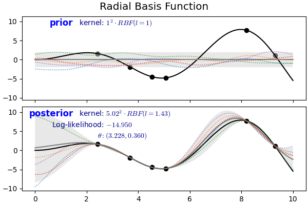
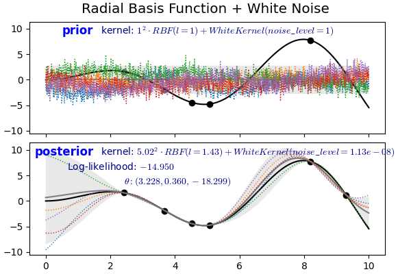
2.2. Radial Basis Function

scikit-learn: RBF Kernel

• Gaussian Process의 가장 기본이 되는 커널입니다.
• 매끈한 곡선이 우리가 알고 있는 가장 기본적인 모양입니다.

  kernel = 1*RBF(length_scale=1.0, length_scale_bounds=(1e-2, 1e2))
  fig = plot_pp(kernel, "Radial Basis Function")

  
  

2.2. White Kernel

scikit-learn: White Kernel

$$k(x_i, x_j) = noise \_ level \text{ if } x_i == x_j \text{ else } 0$$

• 단독으로 사용되기보다 다른 커널에 더해져 노이즈 레벨을 측정하는데 활용됩니다.
• 아래 예제에서는 RBF와의 합으로 사용되었으며, posterior에서 noise level = $1.13 \times 10^{-8}$에 불과합니다.
• prior의 noise level이 데이터를 만나 0에 가깝게 수렴한 것입니다.

  from sklearn.gaussian_process.kernels import WhiteKernel
  
  kernel = 1*RBF(length_scale=1.0, length_scale_bounds=(1e-2, 1e2)) + WhiteKernel(noise_level=1, noise_level_bounds=(1e-8, 1e1))
  fig = plot_pp(kernel, "Radial Basis Function + White Noise")

  
  

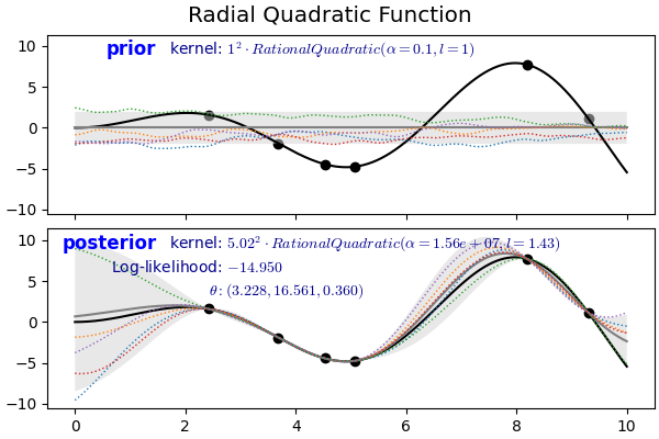
2.3. Radial Quadratic Kernel

scikit-learn: Rational Quadratic Kernel

$$k(x_i, x_j) = \left(1 + \frac{d(x_i, x_j)^2 }{ 2\alpha l^2}\right)^{-\alpha}$$

• RBF Kernel과 다른 거리 스케일링의 혼합 척도(scale mixture)로 볼 수 있습니다.
• prior에서는 RBF 커널에 비해 곧게 펴진 듯한 모습이지만 posterior는 RBF와 잘 구분되지 않습니다.

  from sklearn.gaussian_process.kernels import RationalQuadratic
  
  kernel = 1.0 * RationalQuadratic(length_scale=1.0, alpha=0.1, alpha_bounds=(1e-5, 1e15))
  fig = plot_pp(kernel, "Radial Quadratic Function")

  
  

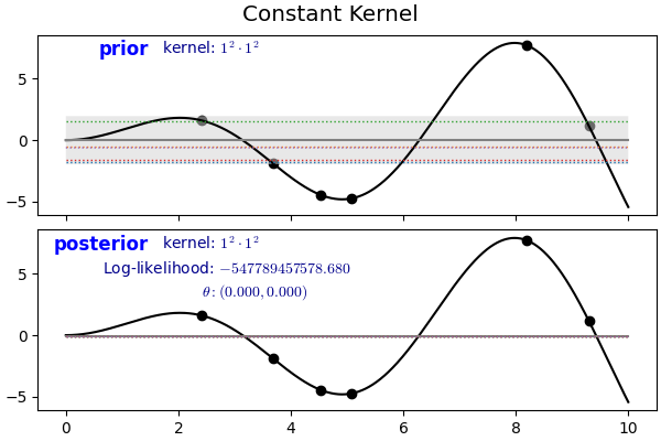
2.4. Constant Kernel

scikit-learn: Constant Kernel

$$k(x_1, x_2) = constant\_value ;\forall; x_1, x_2$$

• 글자 그대로 상수 커널입니다.
• White Kernel과 유사하게 다른 커널과 함께 사용됩니다.

  from sklearn.gaussian_process.kernels import ConstantKernel
  
  kernel = 1.0 * ConstantKernel(constant_value=1.0, constant_value_bounds=(1e-5, 1e15))
  fig = plot_pp(kernel, "Constant Kernel")

  
  

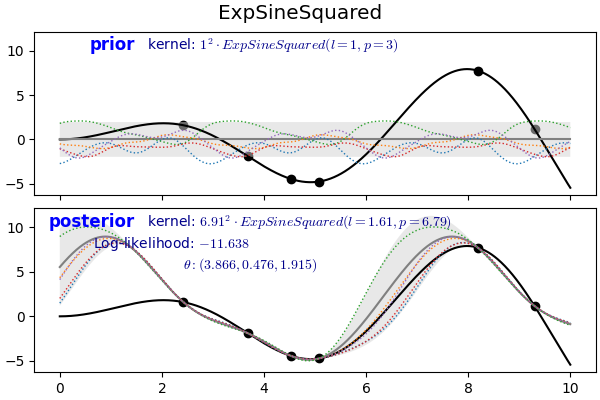
2.5. Exp-Sine-Squared Kernel (periodic kernel)

scikit-learn: ExpSineSquared

$$k(x_i, x_j) = \text{exp}\left(-\frac{ 2\sin^2(\pi d(x_i, x_j)/p) }{ l^ 2} \right)$$

• 지수함수에 sine함수의 제곱이 포함된 형태입니다.
• 주기성을 갖는 데이터를 묘사하기 좋으며 length scale $l > 0$과 함께 periodicity $p > 0$를 매개변수로 가집니다.
• $p$는 Euclidean distance입니다.
• prior와 posterior 모두 자세히 보면 주기성을 띄고 있습니다.

  from sklearn.gaussian_process.kernels import ExpSineSquared
  
  kernel = 1.0 * ExpSineSquared(
      length_scale=1.0,
      periodicity=3.0,
      length_scale_bounds=(0.1, 10.0),
      periodicity_bounds=(1.0, 10.0),
  )
  fig = plot_pp(kernel, "ExpSineSquared")

  
  

2.6. Dot Product

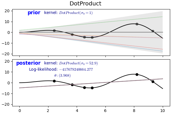
scikit-learn: Dot Product

$$k(x_i, x_j) = \sigma_0 ^ 2 + x_i \cdot x_j$$

• 앞에서 본 커널들은 형태는 달라도 두 점 사이의 거리 $d(x_i, x_j)$를 주요 인자로 가집니다.

• 이런 커널을 stationary kernel이라고 합니다.

• 반면 $x_i$, $x_j$ 값 자체에 의해 좌우되는 커널을 non-stationary kernel이라고 합니다.

• dot product로 정의되기 때문에 원점으로부터의 회전에는 무관하지만 transition에는 민감하게 반응합니다.

• $\sigma_0 = 0$이라면 homogeneous linear kernel, $\sigma_0 \neq 0$이라면 inhomogeneous가 됩니다.

  # 1st degree
  from sklearn.gaussian_process.kernels import DotProduct
  
  kernel = DotProduct(sigma_0=1.0, sigma_0_bounds=(0.1, 100.0))
  fig = plot_pp(kernel, "DotProduct")

  
  

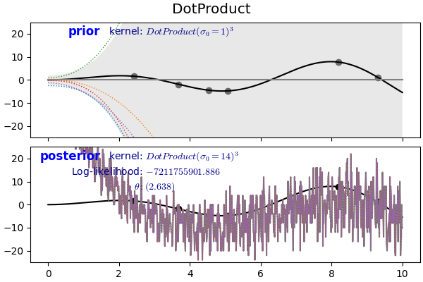
• 제곱식을 통해 다항식을 만들 수 있습니다.

  # 3rd degree
  kernel = DotProduct(sigma_0=1.0, sigma_0_bounds=(0.1, 100.0))**3
  fig = plot_pp(kernel, "DotProduct")
  fig.axes[1].set_ylim(-25, 25)

  
  

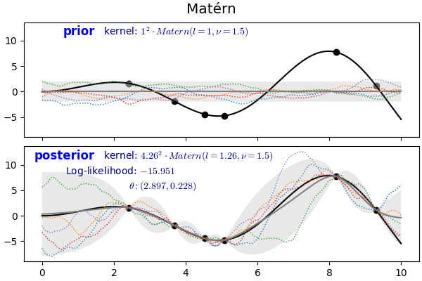
2.7. Matérn Kernel

scikit-learn: Matern

$$k(x_i, x_j) = \frac{1}{\Gamma(\nu)2^{\nu-1}}\Bigg(\frac{\sqrt{2\nu}}{l} d(x_i , x_j )\Bigg)^\nu K_\nu\Bigg(\frac{\sqrt{2\nu}}{l} d(x_i , x_j )\Bigg)$$

• RBF의 일반화된 버전입니다.
• $\nu$로 결과 함수의 smoothness를 조절하는데 $\nu$가 $\infty$에 접근할수록 RBF에 가까워집니다.
• 위 식의 $K_{\nu}(\cdot)$는 modified Bessel function, $\Gamma(\cdot)$는 gamma function입니다.

  from sklearn.gaussian_process.kernels import Matern
  
  kernel = 1.0 * Matern(length_scale=1.0, length_scale_bounds=(1e-1, 10.0), nu=1.5)
  fig = plot_pp(kernel, "Matérn")

  
  

3. 결론

• Gaussian Process는 임의의 적은 데이터로 멋진 결과물을 만들어내지만 Kernel function에 크게 좌우됩니다.
• 문제의 성격과 데이터의 특성에 맞는 적절한 Kernel 선택이 매우 중요합니다.