Shadow Pattern Modeling

2020-10-14

2020-11-27

태양의 일주운동에 따른 건물 그림자 모델 논문을 구현했습니다.
pysolar를 이용해 태양의 운동을 계산하고, geopandas를 이용해 그림자 형상을 계산했습니다.

1. 논문 간단 요약

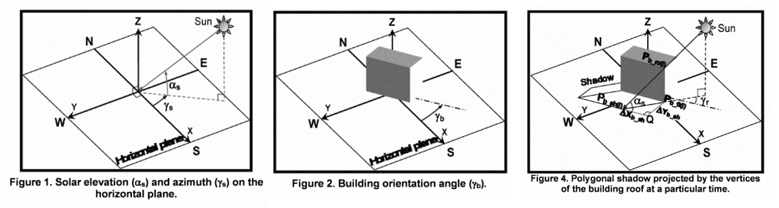
R. Soler-Bientz et al., “Developing a computational tool to assess shadow pattern on a horizontal plane, preliminary results”, IEEE Photovoltaic Specialists Conference p.2312, 2010. doi:10.1109/PVSC.2010.5614490

태양은 아침에 동쪽에서 떠서 남쪽 하늘을 따라 움직이다 저녁이 되면 서쪽으로 넘어갑니다.
태양광은 아주 멀리서 직진하므로 건물이 만드는 그림자는 태양의 좌표와 건물의 형상으로 구할 수 있습니다.

이 둘을 조합하면 위도와 경도가 다른 지구상 여러 위치에서 건물 그림자를 계산할 수 있습니다.

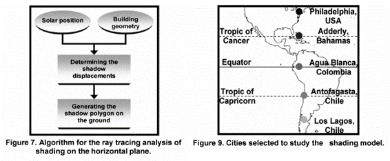
거의 같은 경도 상에 있는 다섯 도시에서 같은 시간에 생기는 그림자를 그려봅니다.
위도에 따라 태양의 위치가 달라 다른 방향과 형태의 그림자가 생깁니다.

2. 태양 일주운동

Pega Devlog: pysolar
pysolar github
ArcGIS: Points Solar Radiation

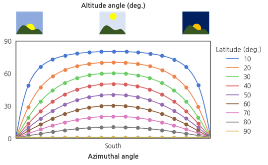
위도와 시간에 따른 태양 고도 변화를 그려봅니다.
춘분(3월 21일) 06시 일출부터 18시 일몰까지 16등분한 태양의 위치입니다.
- arcgis에서 360도를 32등분 하더군요.

방위각azimuthal angle과 고도altitude로 그렸습니다.

import datetime
from pysolar.solar import get_altitude, get_azimuth

lats = list(range(0, 100, 10))
lon = 127.3845

# Spring equinox
KST = datetime.timezone(datetime.timedelta(hours=9))
date = datetime.datetime(2017, 3, 21, 13, 0, 0, tzinfo=KST)

# data
nlats = len(lats)
alts_lat = {}
azis_lat = {}
date_hr_lat = {}

# altitudes and azimuthal angles
for i, lat in enumerate(lats):
    alts, azis, dates_hr = [], [], []
    for hh in range(24):
        for mm in range(0, 60, 1):
            date_hr = datetime.datetime(2017, 3, 21, hh, mm, 0, tzinfo=KST)
            dates_hr.append(date_hr)
            alt = get_altitude(lat, lon, date_hr)
            azi = get_azimuth(lat, lon, date_hr)
            alts.append(alt)
            azis.append(azi)

    date_hr_lat[i] = dates_hr
    alts_lat[i] = np.array(alts)      
    azis_lat[i] = np.array(azis)

hhmm = list(range(1440))    

df_azialt = {}
select_values = np.linspace(90, 270+11.25, 18)
azis_arcgis = {}
alts_arcgis = {}

for i, lat in enumerate(lats):
    df_azialt[i] = pd.DataFrame({"date_hr":hhmm, "azimuth":azis_lat[i], "altitude":alts_lat[i]})
    pcut = pd.cut(df_azialt[i]["azimuth"], select_values)
    azis_arcgis[i] = df_azialt[i]["azimuth"].groupby(pcut).nth(0).values
    alts_arcgis[i] = df_azialt[i]["altitude"].groupby(pcut).nth(0).values

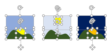
삽입할 그림을 파워포인트에서 도형으로 그립니다.
matplotlib의 .add_axes()를 사용해 그림을 넣을 위치를 지정합니다.

그림 삽입 후 .axis("off")로 가로 세로 눈금을 떼어버립니다.

from matplotlib.ticker import MultipleLocator

fig, ax = plt.subplots(figsize=(10, 10))
lines = []

for i in range(1, nlats):
    line = ax.plot(azis_lat[i], alts_lat[i], zorder=1)
    lines.append(line)
    ax.scatter(azis_arcgis[i], alts_arcgis[i], zorder=1.1)
    
ax.set_aspect("equal")
ax.set_xlim(90, 270)  
ax.set_ylim(0, 90)

xticklabels = [""]*len(ax.get_xticks())
xticklabels[0] = "East"
xticklabels[int(len(ax.get_xticks())/2)] = "South"
xticklabels[-1] = "West"
ax.set_xticklabels(xticklabels)
ax.set_xlabel("Azimuthal angle", fontdict={"fontweight":"bold"}, labelpad=12)
ax.set_title("Altitude angle (deg.)", fontdict={"fontweight":"bold"}, pad=90)
ax.yaxis.set_major_locator(MultipleLocator(30))

plt.legend(lats[1:], bbox_to_anchor=(1,1), frameon=False, title="Latitude (deg.)")

im_sunrise = plt.imread("sunrise.png")
ax_sunrise = fig.add_axes([0.06, 0.69, 0.1, 0.1], anchor="NW", zorder=2)
ax_sunrise.imshow(im_sunrise)
ax_sunrise.axis("off")

im_suntop = plt.imread("suntop.png")
ax_suntop = fig.add_axes([0.37, 0.69, 0.1, 0.1], anchor="NW", zorder=2)
ax_suntop.imshow(im_suntop)
ax_suntop.axis("off")


im_sunset = plt.imread("sunset.png")
ax_sunset = fig.add_axes([0.68, 0.69, 0.1, 0.1], anchor="NW", zorder=2)
ax_sunset.imshow(im_sunset)
ax_sunset.axis("off")

fig.tight_layout()

3. 건물 그리기

Pega Devlog: Create Shapefile from Polygon Dots
Pega Devlog: Mapping Shapefile on Raster Map
geopandas: GeoDataFrame

좌표로 사각형을 만드는 함수입니다.

지난 글에서는 파일로 저장했지만 이번엔 메모리에 올려서 사용합니다.

import geopandas as gpd
from shapely.geometry import MultiPoint

def create_rec(x, y, width, length, angle):
    l_half = length/2
    w_half = width/2
    a_rad = np.deg2rad(angle)
    
    def get_coord(l_half, w_half, a_rad):
        X = x + l_half * np.sin(a_rad) - w_half * np.cos(a_rad)
        Y = y + l_half * np.cos(a_rad) + w_half * np.sin(a_rad)
        return (X, Y)
    
    points = [get_coord(l_half, w_half, a_rad),
              get_coord(-l_half, w_half, a_rad),
              get_coord(-l_half, -w_half, a_rad),
              get_coord(l_half, -w_half, a_rad)
             ]
    
    rec = gpd.GeoDataFrame({"points":[points], "geometry":[MultiPoint(points).convex_hull]})
    return rec

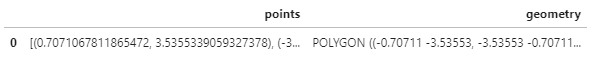
이렇게 만들어진 도형은 geopandas의 GeoDataFrame입니다.
GeoDataFrame은 geometry와 함께 다른 데이터를 담을 수 있습니다.
1
2
rec = create_rec(0, 0, 4, 6, 45)
rec

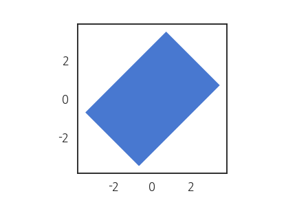
그린 건물을 확인합니다.

1 2	fig, ax = plt.subplots() rec.plot(ax=ax)

4. 그림자 그리기

4.1. 도시별, 시간별 태양 위치

wikipedia: Coordinated Universal Time
python: datetime

그림자는 태양 위치와 건물 모양의 결과물입니다.
- 태양의 위치는 시간에 대한 함수로 주어집니다.
- 그리고 시간은 협정 세계시에 따라 위치별로 다릅니다.

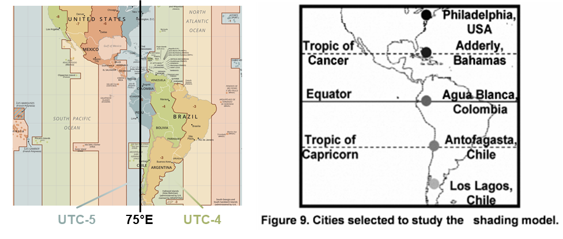
논문에서 제시한 5개 도시는 거의 동경 75도상에 위치합니다.
그러나 적용 시간대가 다릅니다.
위의 세 도시는 UTC-5, 아래 두 도시는 UTC-4를 따릅니다.
도시별 데이터를 만들어 줍니다.
Antofagasta와 Los Lagos는 UTC-4입니다.
그러나 논문 결과는 UTC-5를 넣어야 구현됩니다.

저자의 실수로 생각됩니다.

cities = ["Philadelphia", "Adderly", "Agua Blanca", "Antofagasta", "Los Lagos"]
lats = [39+57/60, 23+36/60, -2/60, -(23+39/60), -(39+51/60)]
lons = [-(75+9/60), -(75+18/60), -(75+12/60), -(72+0/60), -(72+50/60)]  # negative for East Longitude
TZs = [-5, -5, -5, -5, -5]  # "Antofagasta", "Los Lagos" 데이터 오류?

각 도시별, 시간대별 태양의 방위각과 고도를 구합니다.

시간도 다르기 때문에 도시별 timezone 설정을 해 줍니다.

### data
nlats = len(lats)
alts_lat = {}
azis_lat = {}
date_hr_lat = {}

### altitudes and azimuthal angles
for i, (lat, lon, TZ) in enumerate(zip(lats, lons, TZs)):
    # timezone
    tz = datetime.timezone(datetime.timedelta(hours=TZ))
    
    alts, azis, dates_hr = [], [], []
    for hh in range(24):
        for mm in range(0, 60, 30):
            date_hr = datetime.datetime(2008, 3, 21, hh, mm, 0, tzinfo=tz)
            dates_hr.append(date_hr)
            alt = get_altitude(lat, lon, date_hr)
            azi = get_azimuth(lat, lon, date_hr)
            alts.append(alt)
            azis.append(azi)

    date_hr_lat[i] = dates_hr
    alts = np.array(alts)      
    alts_lat[i] = alts
    azis = np.array(azis)
    azis_lat[i] = azis

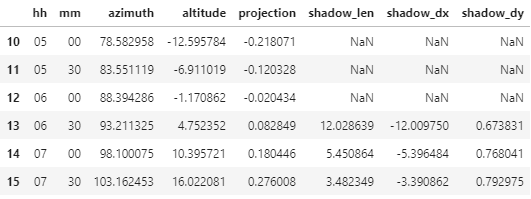
결과를 dataframe으로 정리합니다.
datetime.strftime()을 사용해 시각과 분을 추출하고

방위각과 고도를 이용해 그림자 끝점을 추출합니다.

df_solars = {}

for i, lat in enumerate(lats):
    df_solar = pd.DataFrame({"hh":[date_hr_lat[i][j].strftime("%H") for j in range(48)],
                             "mm":[date_hr_lat[i][j].strftime("%M") for j in range(48)],
                             "azimuth": azis_lat[i],
                             "altitude": alts_lat[i],
                             "projection": np.sin(np.deg2rad(alts_lat[i]))
                            })
    df_solar["shadow_len"] = df_solar["altitude"].apply(lambda x: 1/np.tan(np.deg2rad(x)) if x > 0 else np.nan)
    df_solar["shadow_dx"] = -df_solar["shadow_len"] * np.sin(np.deg2rad(df_solar["azimuth"]))
    df_solar["shadow_dy"] = -df_solar["shadow_len"] * np.cos(np.deg2rad(df_solar["azimuth"]))
    
    df_solars[i] = df_solar

데이터를 확인해 봅니다.
1
df_solars[0].loc[10:15]

4.2. 그림자 그리기 함수

pandas: styling

상자 모양 건물의 그림자를 그립니다.
- 네 꼭지점에서 각기 그림자 포인트를 찾고
- 건물 밑의 네 꼭지점을 연결합니다.
앞에서 구해둔 데이터프레임을 이용합니다.

shadow_dx, shadow_dy를 적용합니다.

def get_shadows(src_x, src_y, src_width, src_length, src_height, src_angle, df_solar):
    # shadow points
    s_points = []
    rec = create_rec(src_x, src_y, src_width, src_length, src_angle)
    points = rec.loc[0, "points"]
    
    for px, py in points:
        sx = px + src_height * df_solar["shadow_dx"].values
        sy = py + src_height * df_solar["shadow_dy"].values
        s_points.append(list(zip(sx, sy)))
    
    shadows_list = []
    for i in range(df_solar.shape[0]):
        mpoints_i = MultiPoint(points + np.array(s_points)[:,i].tolist())
        shadows_list.append(mpoints_i)
    
    shadows = gpd.GeoDataFrame({"geometry":shadows_list})
    return shadows

테스트를 해 봅니다.

1 2	shadows_test1 = get_shadows(0, 0, 4, 6, 8, 45, df_solars[0]) shadows_test1.head()

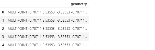
그림으로 그려봅니다.
1
shadows_test1.loc[17, "geometry"]

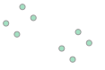
오른쪽 네 개의 점은 바닥면 점,
왼쪽 네 개의 점은 윗면이 만든 그림자 점입니다.
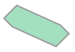
위 함수 15번째 줄에 convex_hull을 넣어 면을 만듭니다.
1
shadows_list.append(mpoints_i.convex_hull)

다시 그려봅니다.

1 2	shadows_test2 = get_shadows(0, 0, 4, 6, 8, 45, df_solars[0]) shadows_test2.loc[17, "geometry"]

앞서 계산한 태양의 이동을 따라 그림자를 그립니다.

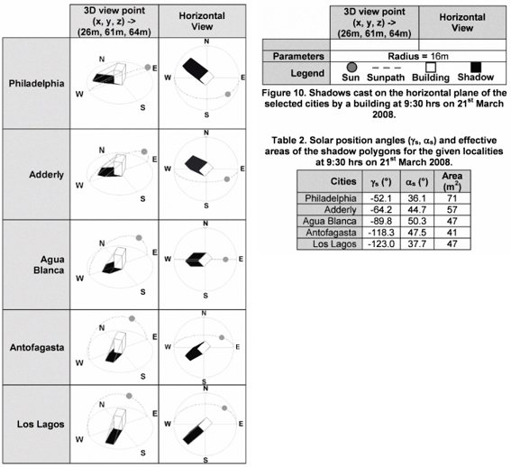
논문에서 제시한 9:30 AM의 그림자를 추가로 그립니다.

from matplotlib.patches import Circle

fig, axes = plt.subplots(ncols=5, nrows=2, figsize=(15, 6))
axs = axes.ravel()

for i in range(5):
    paper_im = plt.imread(f"paper_{i}.png")
    axs[i].imshow(paper_im)
    axs[i].set_xticks([])
    axs[i].set_yticks([])
    [axs[i].spines[k].set_edgecolor("lightgray") for k in axs[i].spines.keys()]
    
    axs[i].set_title(cities[i], fontdict={"fontweight":"bold"}, pad=16)
    
    if i == 0:
        axs[i].set_ylabel("Soler-Bientz\net al.", rotation=0, labelpad=56, 
                          fontdict={"fontweight":"bold", "ha":"center", "va":"center"})

for i in range(5, 10):
    shadow = get_shadows_2(0, 0, 4, 6, 8, 45, df_solars[i-5])
    shadow.plot(ax=axs[i], facecolor="gray", edgecolor="w", alpha=0.1, zorder=1)
    shadow_930.idx = df_solars[i-5].loc[df_solars[i-5]["hh"] == "09"].loc[df_solars[i-5]["mm"] == "30"].index[0]
    shadow_930 = gpd.GeoDataFrame({"geometry":[shadow.loc[19, "geometry"]]})
    shadow_930.plot(ax=axs[i], facecolor="gray", edgecolor="k", linewidth=1, zorder=2)
    rec.plot(ax=axs[i], zorder=3, facecolor="w", edgecolor="k", linewidth=1)
    axs[i].set_xlim(-21, 21)
    axs[i].set_ylim(-21, 21)
    axs[i].set_xticks([])
    axs[i].set_yticks([])
    [axs[i].spines[k].set_edgecolor("lightgray") for k in axs[i].spines.keys()]
    
    # patches
    circle = Circle((0, 0), 15, linewidth=0.5, edgecolor="gray", fill=False)
    axs[i].add_patch(circle)
    axs[i].plot([-15, 15], [0, 0], linewidth=0.5, color="gray" )
    axs[i].plot([0, 0], [-15, 15], linewidth=0.5, color="gray" )
    
    # annotates
    axs[i].annotate("W", (-17.5, 0), ha="center", va="center", fontsize="12", fontweight="bold")
    axs[i].annotate("E", (17.5, 0), ha="center", va="center", fontsize="12", fontweight="bold")
    axs[i].annotate("S", (0, -17.5), ha="center", va="center", fontsize="12", fontweight="bold")
    axs[i].annotate("N", (0, 17.5), ha="center", va="center", fontsize="12", fontweight="bold")
    
    if i == 5:
        axs[i].set_ylabel("Jehyun Lee\n(Pega)", rotation=0, labelpad=56, 
                          fontdict={"fontweight":"bold", "ha":"center", "va":"center"})

fig.align_ylabels([axs[0], axs[5]])            
fig.tight_layout()

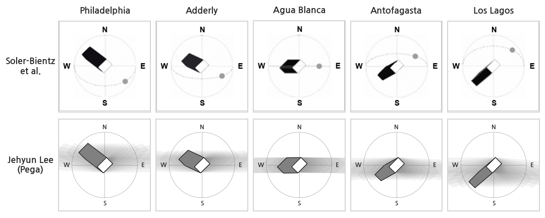
논문 그림이 거의 똑같이 재현되었습니다.

태양 방위각, 고도와 그림자 넓이를 수치로 비교합시다.

# shadow area at 9:30
azis_summary = []
alts_summary = []
areas_summary = []

for i in range(nlats):
    azi = df_solars[i].loc[19, "azimuth"]
    alt = df_solars[i].loc[19, "altitude"]
    shadow = get_shadows_2(0, 0, 4, 6, 8, 45, df_solars[i])
    shadow_930 = gpd.GeoDataFrame({"geometry":[shadow.loc[19, "geometry"]]})
    
    azis_summary.append(azi-180)
    alts_summary.append(alt)
    areas_summary.append(shadow_930.area.values[0] - 24)
    
df_summary = pd.DataFrame({"Cities": cities, 
                           "azimuth (deg.)": azis_summary, 
                           "altitude (deg.)": alts_summary, 
                           "area (m2)": areas_summary})

df_summary.style.format({"azimuth (deg.)":"{:.1f}",
                         "altitude (deg.)":"{:.1f}",
                         "area (m2)":"{:.0f}"})

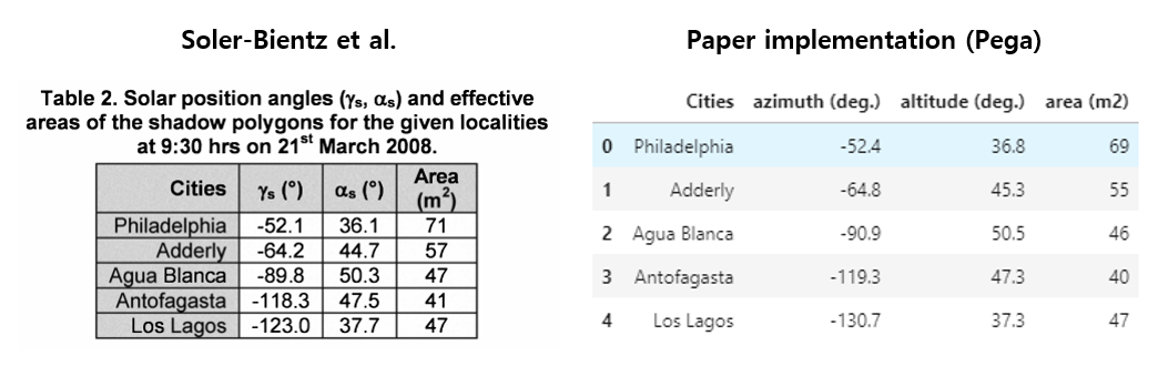
수치적으로도 거의 똑같이 재현되었습니다.

도움이 되셨나요? 카페인을 투입하시면 다음 포스팅으로 변환됩니다

GISPython