Validation with Visualization (2)

2021-04-04

2022-02-06

machine learning, matplotlib, python, sklearn, visualization

contributor: 김홍비님

지난 글에 이어 GridSearchCV를 시각화해봅니다.
화면이라는 매체의 제약상 한 번에 두 개의 변수밖에 바꾸지 못합니다.
그런데도 제법 속이 뚫리고 다음에 뭘 할지 아이디어가 생깁니다.

4. 비선형 모델: kernel SVM

sklearn: svm.SVR

선형 모델로는 한계가 있는 것 같습니다.
비선형성을 가미해봅시다.
Support Vector Machine은 선형 모델이지만 비선형 커널을 함께 사용할 수 있습니다.

파이프라인의 선형회귀를 SVR로 교체합니다.

SVR에 비선형 관련 매개변수가 들어갑니다:
kernel='rbf', gamma=1, C=0.1을 넣어봅니다.

코드 보기/접기

from sklearn.svm import SVR

def svr(degree):
    
    # categorical and numerical features
    cat_features = ["A", "D"]
    cat_transformer = OneHotEncoder(sparse=False)
    
    num_features = ["B", "C", "E"]
    num_transformer = Pipeline(steps=[("scaler", StandardScaler()),
                                      ("polynomial", PolynomialFeatures(degree=degree, 
                                                                        include_bias=True))])
    
    # preprocessor
    preprocessor = ColumnTransformer(transformers=[("num", num_transformer, num_features),
                                                   ("cat", cat_transformer, cat_features)
                                                  ])
    
    # modeling
    model = Pipeline(steps=[("preprocessor", preprocessor), 
                            ("svr", SVR(kernel="rbf", gamma=1, C=0.1)) # 이 부분입니다.
                           ])
    
    return model

SVR의 cross validation plot을 그려봅니다.

method 매개변수를 넣어서 선형회귀와 SVR을 선택할 수 있게 합니다.

코드 보기/접기

def plot_cv(X_train, y_train, title, method="linear"):
    fig, axs = plt.subplots(ncols=3, figsize=(12, 5))

    for degree in range(1, 6):
        # model build
        if method == "linear":
            model = linear(degree)
        elif method == "svr":
            model = svr(degree)

        # cross validation
        for scoring, ax in zip(["neg_mean_absolute_error", "neg_mean_squared_error", "r2"], axs):
            scores = cross_val_score(model, X_train, y_train, scoring=scoring, cv=10)
            if scoring.startswith("neg_"):
                scores = -scores

            cvs = ax.bar(degree, scores.mean()) 
            ax.bar_label(cvs, fmt="%.2f", fontsize=14, padding=5)
            ax.errorbar(degree, scores.mean(), yerr=scores.std(), 
                        ecolor="darkgray", capsize=5, capthick=2)

    for title_, ax in zip(["MAE", "RMSE", "R2"], axs):
        ax.set_title(title_, pad=12)
        ax.grid(axis="y", c="lightgray", ls=":")
        xticks = list(range(1, 6))
        ax.set_xticks(xticks)
        ax.set_xticklabels(xticks)

    fig.suptitle(f"{title}", fontsize=24)
    fig.tight_layout()
    fig.set_facecolor("w")
    fig.savefig(f"{title.replace('(', '_').replace(')', '_').replace(':', '_')}.png")

1	plot_cv(X_train, y_train, "SVR: polynomial order vs metrics (cross validation)", method="svr")

![](SVR_ polynomial order vs metrics _cross validation_.png)

1차의 경우 선형회귀보다 나은 것 같습니다.
파라미터를 바꾸면 더 좋아지지 않을까요?

SVC 파라미터를 바꿀 수 있도록 코드를 조금 수정합니다.

코드 보기/접기

def svr(degree, **kwargs):  # **kwargs로 keyword arguments를 넣을 수 있도록 고칩니다.
    
    # categorical and numerical features
    cat_features = ["A", "D"]
    cat_transformer = OneHotEncoder(sparse=False)
    
    num_features = ["B", "C", "E"]
    num_transformer = Pipeline(steps=[("scaler", StandardScaler()),
                                      ("polynomial", PolynomialFeatures(degree=degree, 
                                                                        include_bias=True))])
    
    # preprocessor
    preprocessor = ColumnTransformer(transformers=[("num", num_transformer, num_features),
                                                   ("cat", cat_transformer, cat_features)
                                                  ])
    
    # modeling
    model = Pipeline(steps=[("preprocessor", preprocessor), 
                            ("svr", SVR(**kwargs))
                           ])
    
    return model

SVC 파라미터에 따른 시각화를 할 수 있도록 수정하고 적용합니다.

C=0.1에서 C=0.2로 바꾼 것만으로 R2가 0.1 정도 상승했습니다.

코드 보기/접기

def plot_cv(X_train, y_train, title, method="linear", **kwargs):
    fig, axs = plt.subplots(ncols=3, figsize=(12, 5))

    for degree in range(1, 6):
        # model build
        if method == "linear":
            model = linear(degree, **kwargs)
        elif method == "svr":
            model = svr(degree, **kwargs)

        # cross validation
        for scoring, ax in zip(["neg_mean_absolute_error", "neg_mean_squared_error", "r2"], axs):
            scores = cross_val_score(model, X_train, y_train, scoring=scoring, cv=10)
            if scoring.startswith("neg_"):
                scores = -scores

            cvs = ax.bar(degree, scores.mean()) 
            ax.bar_label(cvs, fmt="%.2f", fontsize=14, padding=5)
            ax.errorbar(degree, scores.mean(), yerr=scores.std(), 
                        ecolor="darkgray", capsize=5, capthick=2)

    for title_, ax in zip(["MAE", "RMSE", "R2"], axs):
        ax.set_title(title_, pad=12)
        ax.grid(axis="y", c="lightgray", ls=":")
        xticks = list(range(1, 6))
        ax.set_xticks(xticks)
        ax.set_xticklabels(xticks)

    fig.suptitle(f"{title}", fontsize=24)
    fig.tight_layout()
    fig.set_facecolor("w")
    fig.savefig(f"{title.replace('(', '_').replace(')', '_').replace(':', '_')}.png")

1 2	plot_cv(X_train, y_train, "SVR2: polynomial order vs metrics (cross validation)", method="svr", kernel="rbf", gamma=1, C=0.2)

![](SVR2_ polynomial order vs metrics _cross validation_.png)

5. GridSearchCV

sklearn: GridSearchCV

매개변수에 따른 교차검증을 자동으로 하는 방법으로 GridSearchCV가 좋습니다.
일반적으로 사용하는 방법을 그대로 사용해보고,
시각적으로 확인하는 방법을 사용해봅니다.

5.1. 일반 활용

GridSearchCV에 어떤 변수를 어떻게 바꿀지 지정합니다.
단독으로 사용할 수도 있고 pipeline을 포함할 수도 있습니다.
평가 지표(metric)를 여러개 넣을 수 있습니다.

그러나 최적 조건으로 다시 학습하는 refit=은 하나를 지정해야 합니다.

코드 보기/접기

from sklearn.model_selection import GridSearchCV

def svr_gscv(degree, param_grid, **kwargs):
    
    # categorical and numerical features
    cat_features = ["A", "D"]
    cat_transformer = OneHotEncoder(sparse=False)
    
    num_features = ["B", "C", "E"]
    num_transformer = Pipeline(steps=[("scaler", StandardScaler()),
                                      ("polynomial", PolynomialFeatures(degree=degree, 
                                                                        include_bias=True))])
    
    # preprocessor
    preprocessor = ColumnTransformer(transformers=[("num", num_transformer, num_features),
                                                   ("cat", cat_transformer, cat_features)
                                                  ])
    
    # modeling
    model = Pipeline(steps=[("preprocessor", preprocessor), 
                            ("svr", SVR(**kwargs))
                           ])
    
    gscv = GridSearchCV(model, param_grid=param_grid, 
                        scoring=["neg_mean_absolute_error", "neg_root_mean_squared_error", "r2"],
                        refit="neg_root_mean_squared_error")
    
    return gscv

gridsearch에 pipeline을 넣었습니다.

pipeline 중 어떤 단계의 변수를 바꿔볼지는 __(underscore 두 개)를 이용해 지정합니다.

param_grid = {"svr__C": [1e-1, 1e0, 1e1, 1e2, 1e3], 
              "svr__gamma": np.logspace(-2, 2, 5)}

gscv = svr_gscv(3, param_grid=param_grid, kernel="rbf")

.best_score_를 입력하면 최고 점수가 나옵니다.
1
gscv.best_score_
- 실행 결과:
  1
  -0.3738050475519511

.best_params_를 입력하면 최적 조건이 나옵니다.
1
gscv.best_params_
- 실행 결과:
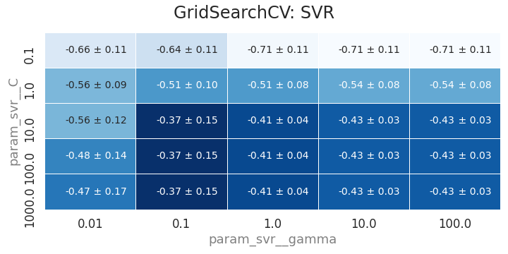
  1
  {'svr__C': 10.0, 'svr__gamma': 0.1}

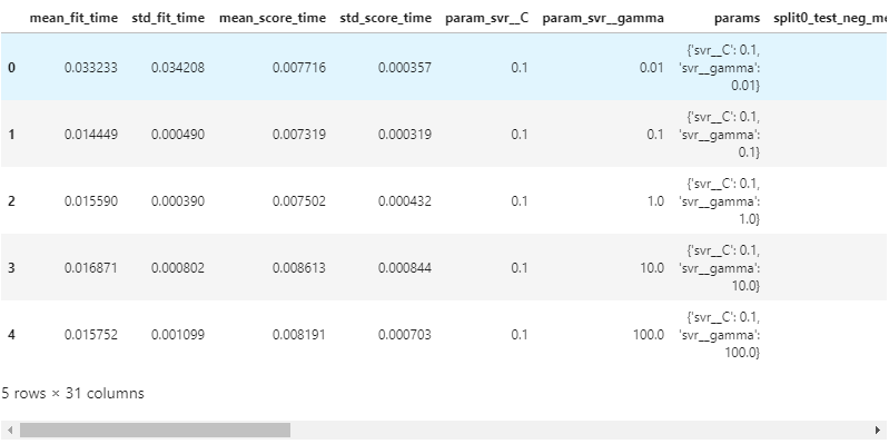
그러나 전체 결과를 보고 싶을 때는 gscv.cv_results_를 사용해 출력하고,
dictionary type이기 때문에 dataframe으로 변환하기 좋습니다.
1
2
df_gscv = pd.DataFrame.from_dict(gscv.cv_results_)
df_gscv.head()

5.2. 시각화

Pega Devlog: Cross Validation with Visualization

5.2.1. 첫 시도

지난 글처럼 평균과 표준편차를 이용해 시각화합시다.
DataFrame을 pivot table로 변환합니다.

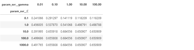
교차검증 평균값을 추출합니다.

1 2	df_pivot_mean = df_gscv.pivot_table(values="mean_test_r2", index="param_svr__C", columns="param_svr__gamma") df_pivot_mean

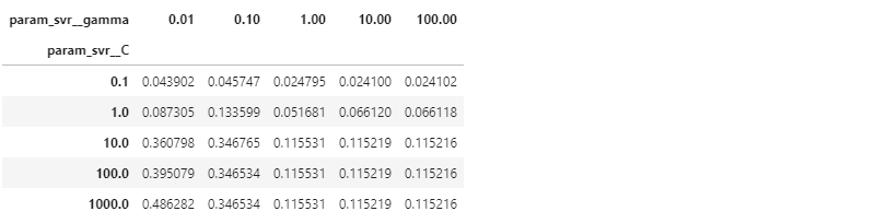
교차검증 표준편차를 추출합니다.

1 2	df_pivot_std = df_gscv.pivot_table(values="std_test_r2", index="param_svr__C", columns="param_svr__gamma") df_pivot_std

평균값과 표준편차를 그림으로 표현합니다.

코드 보기/접기

fig, ax = plt.subplots(figsize=(10, 5))
sns.heatmap(df_pivot_mean, cmap="Blues", lw=1, cbar=False, 
            annot=True, annot_kws={"fontsize":14, "ha":"right"},
            ax=ax)

xticks = ax.get_xticks()
yticks = ax.get_yticks()

font_labels = {"fontsize": 18, "color":"gray"}
ax.set_xlabel("param_svr__gamma", fontdict=font_labels)
ax.set_ylabel("param_svr__C", fontdict=font_labels)

idx_text = 1
for idx, y in zip(df_pivot_std.index, yticks):
    for col, x in zip(df_pivot_std.columns, xticks):
        fontcolor = ax.get_children()[idx_text].get_color()
        ax.text(x, y, f" ± {df_pivot_std.loc[idx, col]:.2f}", 
                color=fontcolor, fontsize=14, va="center")   
        idx_text += 1
        

fig.tight_layout()
fig.savefig("gscv_svr.png")

![](gscv_svr.png)

.best_params_를 사용해 출력하면 하나의 값만 나옵니다.
그러나 시각화를 하면 앞뒤의 경향이 보이고, 거의 일정한 구간도 보입니다.
코드를 함수화하고 interactive하게 그림을 그리면서 최적 조건을 찾아봅니다.

5.2.2. 함수화

GridSearchCV와 heatmap 시각화를 동시에 하는 코드를 작성합니다.

코드 보기/접기

def plot_gscv_svr(X_train, y_train, param_grid, plot_x, plot_y, plot_metric, plot_title=None, 
                  exp_x=False, exp_y=False, figsize=(10, 5)):
    
    # grid search for SVR
    def svr_gscv(param_grid):
        # categorical and numerical features
        cat_features = ["A", "D"]
        cat_transformer = OneHotEncoder(sparse=False)

        num_features = ["B", "C", "E"]
        num_transformer = Pipeline(steps=[("scaler", StandardScaler()),
                                          ("polynomial", PolynomialFeatures(include_bias=True))])

        # preprocessor
        preprocessor = ColumnTransformer(transformers=[("num", num_transformer, num_features),
                                                       ("cat", cat_transformer, cat_features)
                                                      ])

        # modeling
        model = Pipeline(steps=[("preprocessor", preprocessor), 
                                ("svr", SVR())
                               ])

        gscv = GridSearchCV(model, param_grid=param_grid, 
                            scoring=["neg_mean_absolute_error", "neg_root_mean_squared_error", "r2"],
                            refit=plot_metric)
        return gscv

    # training
    gscv = svr_gscv(param_grid)
    gscv.fit(X_train, y_train)
    
    # grid search results summary
    df_gscv = pd.DataFrame.from_dict(gscv.cv_results_)
    
    # creating pivot table
    df_pivot_mean = df_gscv.pivot_table(values=f"mean_test_{plot_metric}", index=plot_y, columns=plot_x)
    df_pivot_std = df_gscv.pivot_table(values=f"std_test_{plot_metric}", index=plot_y, columns=plot_x)
    
    # visualization
    def plot_gscv(df_pivot_mean, df_pivot_std, plot_title):
        fig, ax = plt.subplots(figsize=figsize)
        sns.heatmap(df_pivot_mean, cmap="Blues", lw=1, cbar=False, 
                    annot=True, annot_kws={"fontsize":14, "ha":"right"},
                    ax=ax)

        xticks = ax.get_xticks()
        if exp_x:
            xticklabels = ax.get_xticklabels()
            ax.set_xticks(xticks)
            ax.set_xticklabels([f"{float(x.get_text()):.1e}" for x in xticklabels])

        yticks = ax.get_yticks()
        if exp_y:
            yticklabels = ax.get_yticklabels()
            ax.set_yticks(yticks)
            ax.set_yticklabels([f"{float(y.get_text()):.2e}" for y in yticklabels], rotation=0)
            ax.tick_params(labelsize=14)

        font_labels = {"fontsize": 18, "color":"gray"}
        ax.set_xlabel(f"{plot_x}", fontdict=font_labels)
        ax.set_ylabel(f"{plot_y}", fontdict=font_labels)

        idx_text = 1
        for idx, y in zip(df_pivot_std.index, yticks):
            for col, x in zip(df_pivot_std.columns, xticks):
                fontcolor = ax.get_children()[idx_text].get_color()
                ax.text(x, y, f" ± {df_pivot_std.loc[idx, col]:.2f}", 
                        color=fontcolor, fontsize=14, va="center")   
                idx_text += 1

        fig.suptitle(f"{plot_title}", fontsize=24)
        fig.tight_layout()
        fig.savefig(f"{plot_title.replace('(', '_').replace(')', '_').replace(':', '_')}.png")
    
    plot_gscv(df_pivot_mean, df_pivot_std, plot_title)
    
    return gscv, df_gscv

이 함수를 이용해 GridSearchCV를 수행합니다.

param_grid = {"preprocessor__num__polynomial__degree": [3],
              "svr__kernel": ["rbf"],
              "svr__C": [1e-1, 1e0, 1e1, 1e2, 1e3], 
              "svr__gamma": np.logspace(-2, 2, 5)}

gscv, df_gscv = plot_gscv_svr(X_train, y_train, param_grid,
                     plot_x="param_svr__gamma", plot_y="param_svr__C", plot_metric="neg_root_mean_squared_error", 
                     plot_title="GridSearchCV: SVR")

![](GridSearchCV_ SVR.png)

최적점 주변으로 C와 gamma 범위를 조정합니다.

param_grid = {"preprocessor__num__polynomial__degree": [3],
              "svr__kernel": ["rbf"],
              "svr__C": np.logspace(0, 3, 7), 
              "svr__gamma": np.logspace(-2, 1, 5)}

gscv, df_gscv = plot_gscv_svr(X_train, y_train, param_grid, exp_x=True, exp_y=True,
                     plot_x="param_svr__gamma", plot_y="param_svr__C", plot_metric="neg_root_mean_squared_error", 
                     plot_title="GridSearchCV: SVR (refine 1)")

![](GridSearchCV_ SVR _refine 1_.png)

한번 더 조정합니다: 최적점을 찾은 것 같습니다.

param_grid = {"preprocessor__num__polynomial__degree": [3],
              "svr__kernel": ["rbf"],
              "svr__C": np.logspace(-0, 5, 6), 
              "svr__gamma": np.linspace(0.3, 0.5, 5)}

gscv, df_gscv = plot_gscv_svr(X_train, y_train, param_grid, exp_x=True, exp_y=True,
                     plot_x="param_svr__gamma", plot_y="param_svr__C", plot_metric="neg_root_mean_squared_error", 
                     plot_title="GridSearchCV: SVR (refine 2)", figsize=(10,5))

![](GridSearchCV_ SVR _refine 2_.png)

parity plot을 그려봅니다.
train과 testset의 R2는 각기 0.985, 0.459입니다.
오버피팅이지만 같은 차수의 선형회귀보다는 R2가 0.1 늘었습니다.
![](SVR _degree=3, rbf_.png)

5.2.3. 마음껏 사용

polynomial의 차수가 2차인 경우도 한번 해봅니다.
이번엔 과정을 동영상으로 캡처했습니다.

2차는 3차일때보다 또 R2가 0.1 정도 상승했습니다.
![](SVR _degree=2, rbf_.png)

2차원이라는 한계로 인해 한번에 변수를 두개씩밖에 못바꾸는 아쉬움이 있습니다.
그럼에도 불구하고 공간상 추세가 보이기 때문에 다음 단계의 아이디어가 생깁니다.
이렇게 계속 찾아가 보겠습니다.

도움이 되셨나요? 카페인을 투입하시면 다음 포스팅으로 변환됩니다

PythonData Science

4. 비선형 모델: kernel SVM

5. GridSearchCV

5.1. 일반 활용

5.2. 시각화

5.2.1. 첫 시도

5.2.2. 함수화

5.2.3. 마음껏 사용