Matplotlib plot colors

2021-02-04

2021-04-25

color, matplotlib, python, visualization

시각화에서 색상은 중요한 요소입니다.
그러나 관성적으로 프로그램이 제공하는 기본값을 사용하는 분들이 많습니다.
matplotlib은 푸짐한 상을 차려놓고 우리를 기다리고 있습니다. 골라봅시다.

1. Example Bed

화면상에서 색상은 대개 RGB 3채널로 구성됩니다.
여기에 불투명도 Alpha가 붙어 RGBA 4채널이 되기도 합니다.
같은 색상도 숫자, Hex code, 이름, 순번등 여러가지로 표현됩니다.
이들을 그려볼 example bed를 준비합니다.

1.1. Sample Data

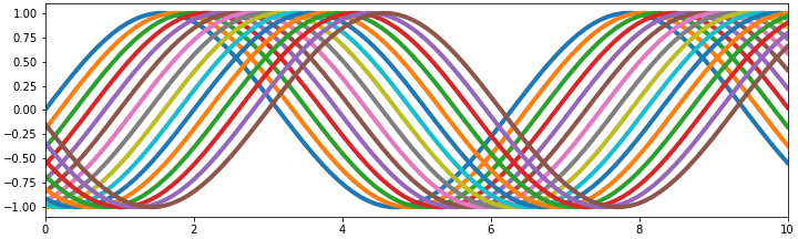
예제 데이터로 sine curve 다발을 사용할 것입니다.

X = np.linspace(0, 10, 100)
size=16

fig, ax = plt.subplots(figsize=(10, 3), constrained_layout=True)

# sine wave plot
for i in range(size):
    ax.plot(X, np.sin(X - 0.2*i), linewidth=4)
    
ax.set_xlim(0, 10)

1.2. Background Image

wikipedia: Lena Forsén(Lena Söderberg)
youtube: Losing Lena
women love tech: Losing Lena – Why Removing One Image Will End Tech’s Original Sin
The USC-SIPI Image Database
wikipedia: Eurasian eagle-owl

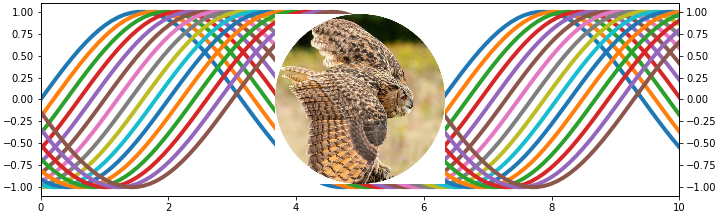
반투명 색상이 잘 표현되는지 확인하기 위해 뒤에 이미지를 깝니다.
이럴 때 Lena Forsén(Lena Söderberg)님의 이미지를 많이 사용했습니다.
그러나 본인이 더 이상 자신의 이미지를 사용하지 않았으면 좋겠다(“I retired from modelling a long time ago, It’s time I retired from tech, too.”)고 하셨기 때문에 의사를 존중해드리려고 합니다.

대신 부엉이를 사용합니다.
유라시안 수리부엉이 사진을 가져와서 넣습니다.

ax.twinx()로 메인 axes와 x축을 공유하는 axes를 만들고, OffsetImage와 AnnotationBbox를 사용해 한가운데 넣습니다.

# image overlay: 위 코드에 추가
from matplotlib.offsetbox import OffsetImage, AnnotationBbox

owl = plt.imread("owl.jpg")    # 배경 이미지 읽어오기
ax_owl = ax.twinx()            # 이미지가 들어갈 axes 만들기
ax_owl.set_xlim(ax.get_xlim())       # 메인 axes와 x범위 통일 : 혼동 방지
ax_owl.set_ylim(ax.get_ylim())       # 메인 axes와 y범위 통일 : 혼동 방지

oi = OffsetImage(owl, zoom=0.3, alpha=1)         # 이미지 삽입 준비
box0 = AnnotationBbox(oi, (5, 0), frameon=False) # 이미지 삽입 좌표 지정, 테두리 삭제
ax_owl.add_artist(box0)                          # 이미지 삽입

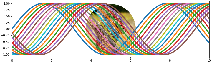
ax_owl.set_zorder(-1)로 순서를 뒤로 옮깁니다.
ax의 기본 zorder는 0이기 때문에 부엉이 그림이 sine 곡선 뒤에 놓입니다.

메인 axes ax를 투명하게 하는 것을 잊지 않습니다.

1
2
3

ax_owl.axis(False)                               # 배경 이미지 눈금 안보이게
ax_owl.set_zorder(-1)                            # 배경 이미지 axes를 메인 axes뒤로
ax.set_facecolor("none")                         # 메인 axes를 투명하게

1.3. function: Color Plot

sine 곡선의 색상을 바꿔가며 그릴 함수를 만듭니다.
입력 인자로 colors(list), title(str)을 의무적으로 받고, style(str)과 prop_cycle(list), 그리고 저장할 파일명을 옵션으로 받게 합니다.
똑같은 sine curve를 colors에 따라 다른 색으로 그릴 것입니다.

style과 prop_cycle은 아래에서 설명하겠습니다.

def plot_color_example(colors, title, style="default", prop_cycle=None, filename=None):
    with plt.style.context(style):
        fig, ax = plt.subplots(figsize=(10,3), constrained_layout=True)

        X = np.linspace(0, 10, 100)
        
        if prop_cycle:
            print(f"# prop_cycle={prop_cycle}")
            ax.set_prop_cycle('color', prop_cycle)
            
        for i, color in enumerate(colors):
            ax.set_facecolor("none")
            ax.set_zorder(2)
            if prop_cycle or style != "default":
                ax.plot(X, np.sin(X-0.2*i), lw=4, label=f"color_{i:02d}")
            else:
                ax.plot(X, np.sin(X-0.2*i), c=color, lw=4, label=color)
            ax.set_title(title, fontsize="large", pad=6)
            ax.legend(ncol=2, loc="upper left", bbox_to_anchor=(1,1))
            ax.set_xlim(0, 10)

        ax_owl = ax.twinx()
        ax_owl.set_zorder(-1)
        ax_owl.set_ylim(-1, 1)
        oi = OffsetImage(owl, zoom = 0.3, alpha=1)
        box0 = AnnotationBbox(oi, (5, 0), frameon=False)
        ax_owl.add_artist(box0)
        ax_owl.axis(False)
        
        if filename:
            fig.savefig(filename)

2. Colors

Matplotlib은 다양한 형태의 색상을 지원합니다.
하나하나 그려보며 확인하겠습니다.

2.1. [0~1]

채널의 강도를 0~1 사이의 숫자를 이용해서 표현합니다.
Grayscale, RGB, Alpha(불투명도)를 표현합니다.

2.1.1. Grayscale

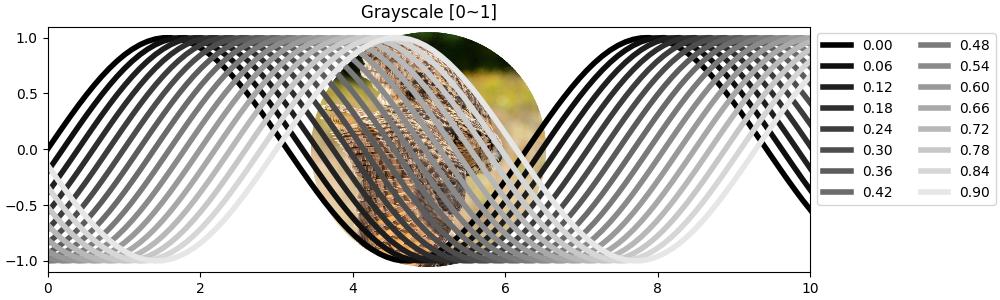
회색조를 0~1 사이 값 str 타입으로 표현할 수 있습니다.

0이 검정, 1이 흰색입니다.

colors = [f"{f:.2f}" for f in np.linspace(0, 0.9, size)]
print(colors)

plot_color_example(colors, "Grayscale [0~1]", filename="mpl_colors_09.png")

실행 결과: 따옴표가 꼭 필요합니다.

1	['0.00', '0.06', '0.12', '0.18', '0.24', '0.30', '0.36', '0.42', '0.48', '0.54', '0.60', '0.66', '0.72', '0.78', '0.84', '0.90']

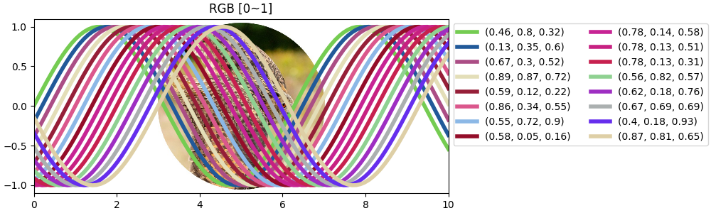
2.1.2. RGB (array)

RGB 각 채널을 0~1 사이 값 float 3개 array로 표현할 수 있습니다.

랜덤으로 색상을 추출했습니다.

colors = [(r.round(2), g.round(2), b.round(2)) for r, g, b
          in zip(np.random.uniform(0, 1, size=size), np.random.uniform(0, 1, size=size), np.random.uniform(0, 1, size=size))]
print(colors)

plot_color_example(colors, "RGB [0~1]", filename="mpl_colors_10.png")

실행 결과: 3차원 array입니다.

[(0.46, 0.8, 0.32), (0.13, 0.35, 0.6), (0.67, 0.3, 0.52), (0.89, 0.87, 0.72), (0.59, 0.12, 0.22), (0.86, 0.34, 0.55), (0.55, 0.72, 0.9), (0.58, 0.05, 0.16), (0.78, 0.14, 0.58), (0.78, 0.13, 0.51), (0.78, 0.13, 0.31), (0.56, 0.82, 0.57), (0.62, 0.18, 0.76), (0.67, 0.69, 0.69), (0.4, 0.18, 0.93), (0.87, 0.81, 0.65)]

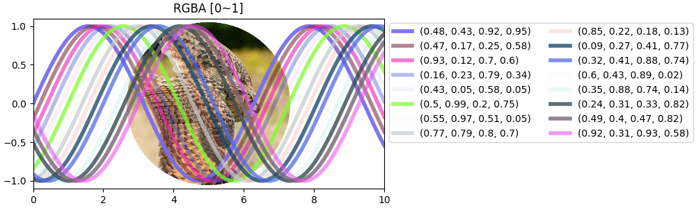
2.1.3. RGBA (array)

RGB에 Alpha(불투명도)채널 하나를 더 추가합니다.

역시 랜덤으로 추출했습니다.

colors = [(r.round(2), g.round(2), b.round(2), a.round(2)) for r, g, b, a 
          in zip(np.random.uniform(0, 1, size=size), np.random.uniform(0, 1, size=size), np.random.uniform(0, 1, size=size), np.random.uniform(0, 1, size=size))]
print(colors)

plot_color_example(colors, "RGBA [0~1]", filename="mpl_colors_11.png")

실행 결과: 4차원 array입니다. 선 너머로 그림이 비칩니다.

[(0.48, 0.43, 0.92, 0.95), (0.47, 0.17, 0.25, 0.58), (0.93, 0.12, 0.7, 0.6), (0.16, 0.23, 0.79, 0.34), (0.43, 0.05, 0.58, 0.05), (0.5, 0.99, 0.2, 0.75), (0.55, 0.97, 0.51, 0.05), (0.77, 0.79, 0.8, 0.7), (0.85, 0.22, 0.18, 0.13), (0.09, 0.27, 0.41, 0.77), (0.32, 0.41, 0.88, 0.74), (0.6, 0.43, 0.89, 0.02), (0.35, 0.88, 0.74, 0.14), (0.24, 0.31, 0.33, 0.82), (0.49, 0.4, 0.47, 0.82), (0.92, 0.31, 0.93, 0.58)]

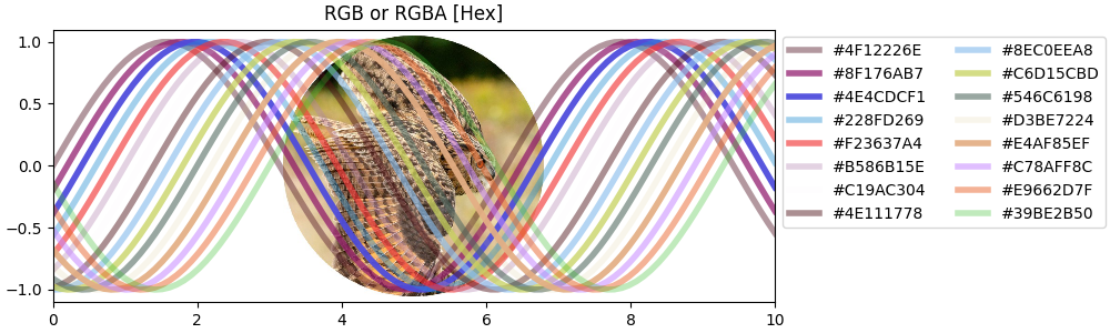
2.1.4. RGB or RGBA (hex)

Pega Devlog: Picking and Modifying Colors
Pega Devlog: Matplotlib colors

RGB 또는 RGBA 형식은 array 외에도 hex code로도 표현됩니다.

대소문자는 구분하지 않습니다.

hex_chrs = [str(i) for i in range(10)]           # 0 ~ 9
hex_chrs.extend([chr(c) for c in range(65, 71)]) # A ~ F
colors = [f"#{r0}{r1}{g0}{g1}{b0}{b1}{a0}{a1}" for r0, r1, g0, g1, b0, b1, a0, a1 
          in zip(np.random.choice(hex_chrs, size=size), np.random.choice(hex_chrs, size=size), np.random.choice(hex_chrs, size=size), np.random.choice(hex_chrs, size=size),
                 np.random.choice(hex_chrs, size=size), np.random.choice(hex_chrs, size=size), np.random.choice(hex_chrs, size=size), np.random.choice(hex_chrs, size=size))]
print(colors)

plot_color_example(colors, "RGB or RGBA [Hex]", filename="mpl_colors_12.png")

실행 결과: # 뒤에 알파벳 6개(RGB) 또는 8개(RGBA)가 오면 됩니다.

[(0.48, 0.43, 0.92, 0.95), (0.47, 0.17, 0.25, 0.58), (0.93, 0.12, 0.7, 0.6), (0.16, 0.23, 0.79, 0.34), (0.43, 0.05, 0.58, 0.05), (0.5, 0.99, 0.2, 0.75), (0.55, 0.97, 0.51, 0.05), (0.77, 0.79, 0.8, 0.7), (0.85, 0.22, 0.18, 0.13), (0.09, 0.27, 0.41, 0.77), (0.32, 0.41, 0.88, 0.74), (0.6, 0.43, 0.89, 0.02), (0.35, 0.88, 0.74, 0.14), (0.24, 0.31, 0.33, 0.82), (0.49, 0.4, 0.47, 0.82), (0.92, 0.31, 0.93, 0.58)]

2.1.5. Utitlities

matplotlib.colors의 to_hex()를 사용하면 array가 hex code로 변경됩니다.
반대 방향은 to_rgb(), to_rgba(), to_rgba_array()로 가능합니다.
어딘가에서 온 array나 string이 matplotlib 색상 표현에 적합한지 알아보는 명령어도 있습니다.

is_color_like입니다.

# check if input is a color
import matplotlib.colors as mcolors

print(f"mcolors.is_color_like((0.16, 0.23, 0.79, 0.34)) = {mcolors.is_color_like((0.16, 0.23, 0.79, 0.34))}")
print(f"mcolors.is_color_like((0.16, 0.23, 0.79, 1.34)) = {mcolors.is_color_like((0.16, 0.23, 0.79, 1.34))}")

print(f"\nmcolors.is_color_like('#4F12226E') = {mcolors.is_color_like('#4F12226E')}")
print(f"mcolors.is_color_like('#4F1226E') = {mcolors.is_color_like('#4F1226E')}")

실행 결과: 1을 넘는 array, 자릿수가 부족한 hex code는 False가 나옵니다.

mcolors.is_color_like((0.16, 0.23, 0.79, 0.34)) = True
mcolors.is_color_like((0.16, 0.23, 0.79, 1.34)) = False

mcolors.is_color_like('#4F12226E') = True
mcolors.is_color_like('#4F1226E') = False

2.2. Strings

Matplotlib에 string으로 저장된 pre-defined color가 있습니다.
네 가지가 있습니다: BASE_COLORS, XKCD_COLORS, CSS4_COLORS, TABLEAU_COLORS입니다.
dictionary 형태로 float array 또는 hex code와 함께 저장되어 있습니다.
1
2
print(type(mcolors.BASE_COLORS))
mcolors.BASE_COLORS

실행 결과:

<class 'dict'>
{'b': (0, 0, 1),
 'g': (0, 0.5, 0),
 'r': (1, 0, 0),
 'c': (0, 0.75, 0.75),
 'm': (0.75, 0, 0.75),
 'y': (0.75, 0.75, 0),
 'k': (0, 0, 0),
 'w': (1, 1, 1)}

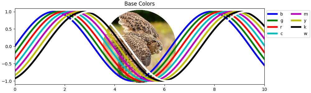
2.2.1. `BASE_COLORS`

영어 한 글자로 색상을 표현합니다.

RGB + CMYK + W 입니다.

1
2
3

colors = list(mcolors.BASE_COLORS.keys())

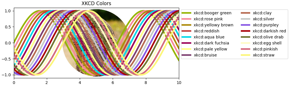
plot_color_example(colors, "Base Colors", filename="mpl_colors_13.png")

2.2.2. `XKCD_COLORS`

list of xkcd colors

954개의 가장 흔히 사용되는 색상에 투표로 이름을 붙였다고 합니다.

역시 랜덤으로 16개만 골랐습니다.

c_xkcd = list(mcolors.XKCD_COLORS.keys())
print(c_xkcd)
colors = np.random.choice(c_xkcd, replace=False, size=size)

plot_color_example(colors, "XKCD Colors", filename="mpl_colors_14.png")

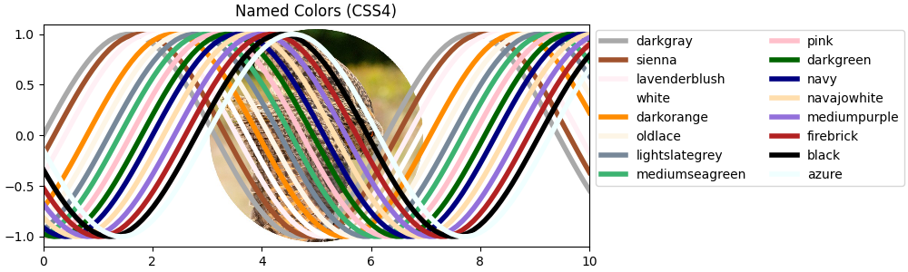
2.2.3. `CSS4_COLORS`: “Named Colors”

matplotlib: List of named colors

저는 색상을 고를 때 이 색상들을 주로 참고하곤 합니다.

세련되고 보기 편한 색상들이 잘 정돈되어 있거든요.

c_css4 = list(mcolors.CSS4_COLORS.keys())
print(c_css4)
colors = np.random.choice(c_css4, replace=False, size=size)

plot_color_example(colors, "Named Colors (CSS4)", filename="mpl_colors_15.png")

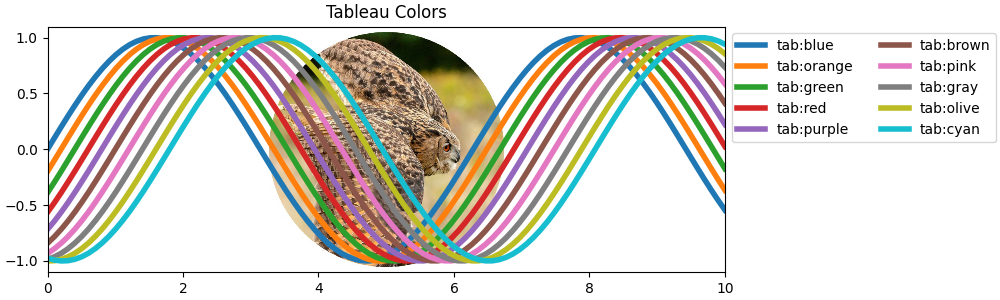
2.2.4. `TABLEAU_COLORS`

matplotlib: what’s new in matplotlib 2.0 > Colors, color cycles, and color maps

데이터 시각화에서 태블로를 빼놓기 어렵습니다.
태블로의 팔레트를 matplotlib에 심었고, matplotlib 버전 2부터 RGBCMWK를 밀어내고 기본 cycle이 되었습니다.
1
2
3
c_tableau = list(mcolors.TABLEAU_COLORS.keys())

plot_color_example(c_tableau, "Tableau Colors", filename="mpl_colors_16.png")

2.3. CN

matplotlib: Specifying Colors
matplotlib: Customizing Matplotlib with style sheets and rcParams

지금의 sine curve 예제처럼 plot을 반복해서 그리면 자동으로 색이 변경됩니다.
matplotlib에서 사용중인 style에 정의된 순환(cycling) 색상들이 순차적으로 적용되는 것입니다.
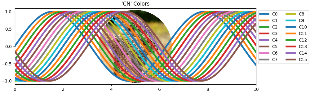
색을 따로 지정하지 않을 경우 첫 plot은 color="C0", 그 다음은 "C1" 이런 식으로 순차적으로 적용되는데, 이를 CN이라고 합니다.
matplotlib 공식 홈페이지에도 CN이 무슨 말의 약자인지는 나와있지 않지만, cycle number로 추정됩니다.

2.3.1. Default: `TABLEAU_COLORS`

논문 그림처럼 복잡한 그림들을 그릴 때 앞에서 사용된 특정 색상을 다시 사용해야 할 때가 있습니다.

이럴 때 CN이 매우 유용합니다.

c_CN = [f"C{i}" for i in range(16)]
print(c_CN)

plot_color_example(c_CN, "'CN' Colors", filename="mpl_colors_17.png")

실행 결과: 기본값은 Tableau와 같습니다. 10개를 상한으로 다시 C0과 같아집니다.

1	['C0', 'C1', 'C2', 'C3', 'C4', 'C5', 'C6', 'C7', 'C8', 'C9', 'C10', 'C11', 'C12', 'C13', 'C14', 'C15']

2.3.2. Palette

Palettable
seaborn: General principles for using color in plots
matplotlib.axes.Axes.set_prop_cycle

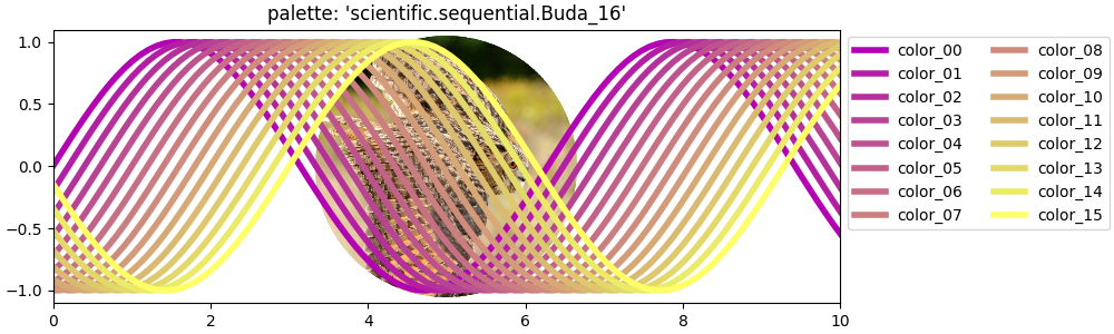
Matplotlib 외부의 팔레트를 가져와 사용할 수 있습니다.
Palettable도 좋고, seaborn도 좋습니다.

ax.set_prop_cycle("color", Palette)형태로 Palette를 지정합니다.

1
2
3

from palettable.scientific.sequential import Buda_16

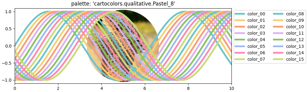
plot_color_example(c_CN, "palette: 'scientific.sequential.Buda_16'", prop_cycle=Buda_16.mpl_colors, filename="mpl_colors_18.png")

여러 가지 선택지가 있습니다.

1
2
3

from palettable.cartocolors.qualitative import Pastel_8

plot_color_example(c_CN, "palette: 'cartocolors.qualitative.Pastel_8'", prop_cycle=Pastel_8.mpl_colors, filename="mpl_colors_19.png")

2.3.3. Colormap

matplotlib: Choosing Colormaps in Matplotlib

colormap에서도 팔레트를 뽑아낼 수 있습니다.
먼저 matplotlib.cm.get_cmap()함수를 사용해서 colormap 객체를 만듭니다.

여기에 괄호로 숫자를 넣어주면 거기에 해당하는 색생이 추출됩니다.

from matplotlib import cm

blues = cm.get_cmap("Blues", lut=size)
c_blues = [blues(i) for i in range(size)]

plot_color_example(c_blues, "colormap: 'Blues'", prop_cycle=c_blues, filename="mpl_colors_24.png")

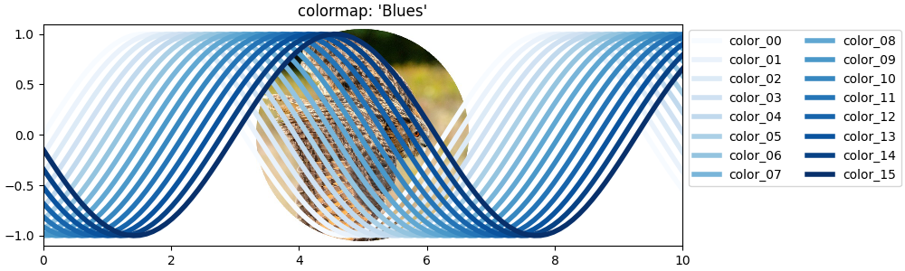
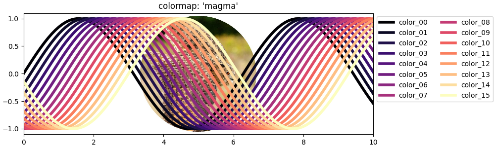
경우의 수가 풍족해집니다.

magma = cm.get_cmap("magma", lut=size)
c_magma = [magma(i) for i in range(size)]

plot_color_example(c_blues, "colormap: 'magma'", prop_cycle=c_magma, filename="mpl_colors_25.png")

2.3.4. style

matplotlib은 style에 글꼴, 색상 등 많은 정보를 담고 있습니다.
style을 바꿔서 cyclic color를 변경할 수 있습니다.

작성중인 코드 전체의 스타일을 바꿀 때는 plt.style.use()를 사용합니다.
임시로 사용하겠다면 with plt.style.context():를 사용합니다.
그런데 plt.style.context()를 사용하면, c=C0 등으로 지정하면 기본 style의 cyclic color가 나옵니다.
색상 자체를 지정하지 않아야 plt.style.context()명령이 의도대로 수행됩니다.

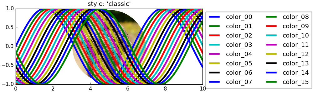
matplotlib 1.x 기본 색상입니다.
1
plot_color_example(c_CN, "style: 'classic'", style="classic", filename="mpl_colors_20.png")

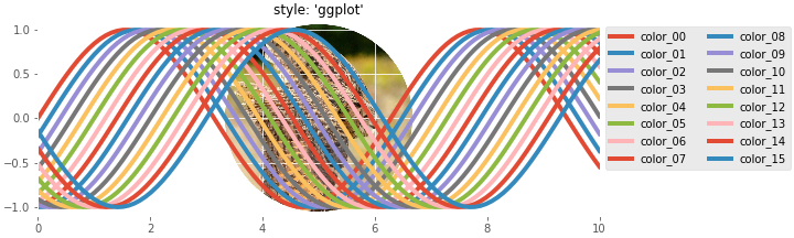
ggplot 스타일도 가능합니다.
1
plot_color_example(c_CN, "style: 'ggplot'", style="ggplot", filename="mpl_colors_21.png")

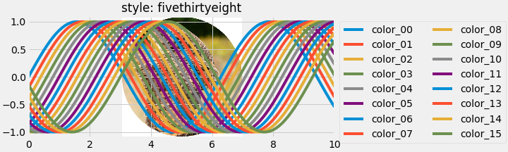
강렬한 fivethirtyeight입니다.
1
plot_color_example(c_CN, "style: fivethirtyeight", style="fivethirtyeight", filename="mpl_colors_23.png")

3. 결론

인지과학적으로 색은 글자보다 먼저 전달되는 정보입니다.

색상만 평소와 다르게 사용하는 것 만으로도 한결 산뜻한 느낌이 들 수 있습니다.

데이터의 성격과 시각화 목적에 더 잘 맞는 색상이라면 말할 것도 없을겁니다.

도움이 되셨나요? 카페인을 투입하시면 다음 포스팅으로 변환됩니다

Share

PythonData Science