Density Plot with Colormap

  • 시각화는 데이터를 그림으로 표현하는 작업입니다.
  • 그런데 한번 그림이 되면 진짜 그림처럼 취급할 수 있습니다.
  • 밀도함수에 컬러맵을 입혀봅시다.

1. Imitating Ridge Plot by R

Gallery of ggridges examples
Pega Devlog: Ridgeline Plot

  • 인터넷을 다니다가 R로 그려진 멋진 그림을 봤습니다.


  • 밀도함수에 컬러맵을 입힌 그림이 멋져서 따라해보고 싶더군요.
  • 저는 R을 사용하지 못하는 파이썬 사용자입니다만 비슷한 그림을 만들었습니다.

  • 코드를 먼저 공개하고 어떻게 한건지 설명하겠습니다.
    1
    2
    3
    4
    5
    6
    7
    8
    9
    10
    11
    12
    13
    14
    15
    16
    17
    18
    19
    20
    21
    22
    23
    24
    25
    26
    27
    28
    29
    30
    31
    32
    33
    34
    35
    36
    37
    38
    39
    40
    41
    42
    43
    44
    45
    46
    47
    48
    49
    50
    51
    52
    53
    54
    55
    56
    57
    58
    59
    60
    61
    62
    63
    64
    65
    import pandas as pd
    import numpy as np
    import matplotlib.pyplot as plt
    import matplotlib as mpl
    import seaborn as sns

    # 네브라스카주 링컨시 데이터 다운: https://github.com/amcquistan/WeatherPredictPythonML
    df_weather = pd.read_csv("end-part2_df.csv", index_col="date")

    # 2016년 데이터만 선택
    df_2016 = df_weather.filter(like="2016", axis=0)

    # 날짜에서 월 추출
    df_2016.reset_index(inplace=True)
    df_2016["month"] = df_2016["date"].apply(lambda s: int(s.split("-")[1]))

    ### 시각화
    import calendar
    import cmocean as cmo

    fig, axs = plt.subplots(nrows=12, figsize=(10,5), sharex=True, sharey=True)
    fig.set_facecolor("none")

    x = np.linspace(0, 1, 100)
    for i, ax in enumerate(axs, 1):
    sns.kdeplot(df_2016.query(f"month=={i}")["meantempm"],
    fill=True, color="w", alpha=0, linewidth=2, legend=False, ax=ax)

    ax.set_xlim(-29, 40)

    # >>> 밀도함수에 gradient 추가
    im = ax.imshow(np.vstack([x, x]),
    cmap="cmo.thermal",
    aspect="auto",
    extent=[*ax.get_xlim(), *ax.get_ylim()]
    )
    path = ax.collections[0].get_paths()[0]
    patch = mpl.patches.PathPatch(path, transform=ax.transData)
    im.set_clip_path(patch)
    # <<< 밀도함수에 gradient 추가

    ax.text(-29, 0.01, calendar.month_name[i], fontdict={"fontsize":"large"})

    ax.spines["left"].set_visible(False)
    ax.spines["right"].set_visible(False)
    ax.spines["top"].set_visible(False)
    ax.spines["bottom"].set_visible(False)
    if i != 12:
    ax.tick_params(axis="x", length=0)
    else:
    ax.tick_params(axis="x", direction="inout", color="lightgray",
    length=5, width=2, labelsize="large")
    ax.set_xlabel("Mean Temperature (℃)", fontdict={"fontsize":"large"})

    ax.set_yticks([])
    ax.set_ylabel("")

    xticks = ax.get_xticks()
    for xtick in xticks:
    ax.plot([xtick, xtick], [0, 0.065], color='lightgray', zorder=0)

    ax.axhline(0, color="lightgray")
    ax.set_facecolor("none")

    fig.subplots_adjust(hspace=-0.5)

2. Colormap on Density Plot

  • 밀도함수에 컬러맵을 얹는 순서는 다음과 같습니다.

1. 밀도함수 그리기: seaborn.kdeplot()
2. 그림 전체에 컬러맵 칠하기: axes.imshow()
3. 밀도함수 영역 따기: matplotlib.collections.get_paths()
4. 컬러맵을 밀도함수 모양에 맞게 자르기: matplotlib.patches.PathPatch(), im.set_clip_path()

  • 한 단계씩 살펴봅니다.

2.1. Sample Data

  • 1월 데이터만 가지고 옵니다.
    1
    2
    df_jan = df_2016.query("month==1")
    df_jan.head()

2.2. 밀도함수 그리기

  • seaborn의 힘을 빌립니다.
  • seaborn.kdeplot()을 사용합니다.
  • fill=True가 중요합니다: matplotlib collection 객체로 만들어야 합니다.
  • alpha=0도 중요합니다: 컬러맵이 잘 표현되도록 배경색을 제거합니다.
    1
    2
    3
    fig, ax = plt.subplots()

    sns.kdeplot(df_jan["meantempm"], fill=True, alpha=0, ax=ax)

2.3. 그림 전체에 컬러맵 칠하기

  • x값을 100단계로 나누어서 이미지를 만듭니다.
  • (2, 100) 형태의 array를 만들어서 그림 크기에 맞게 붙입니다.
    1
    2
    3
    4
    5
    6
    7
    8
    9
    x = np.linspace(0, 1, 100)

    im = ax.imshow(np.vstack([x, x]),
    cmap="inferno",
    aspect="auto",
    extent=[*ax.get_xlim(), *ax.get_ylim()]
    )

    display(fig)

2.4. 밀도함수 영역 따기

matplotlib.collections
matplotlib Tutorials: Path tutorial

  • Matplotlib에는 collection이라는 개념이 있습니다.
  • 여러 도형들을 한데 묶어 관리하는 것으로, 색상이나 선 굵기 등을 한번에 조정할 수 있습니다.
  • 파워포인트의 그룹을 생각하시면 비슷할 듯 합니다.

  • 우리 axes 위에는 방금 그린 밀도함수 뿐이므로, ax.collections객체가 단 하나입니다.

  • 이 객체의 윤곽선을 get_path()명령으로 추출합니다.

    1
    print(ax.collections[0].get_paths()[0])
  • 실행 결과

    1
    2
    3
    4
    5
    Path(array([[-2.48238595e+01,  5.51614084e-05],
    [-2.48238595e+01, 0.00000000e+00],
    [-2.46296499e+01, 0.00000000e+00],
    [-2.44354402e+01, 0.00000000e+00],
    (생략)
  • get_path()의 결과로 두 가지 데이터가 나옵니다.

  • 첫번째는 path의 꼭지점들(vertices) 좌표이고, 두번째는 꼭지점들의 속성입니다.

  • 자세한 사항은 Path Tutorial에서 볼 수 있습니다. 지금은 넘어갑니다.

  • 꼭지점만 받아서 그림을 그려도 밀도함수의 윤곽선이 나옵니다.

    1
    2
    3
    vertices = ax.collections[0].get_paths()[0].vertices.T

    plt.plot(*vertices)


2.5. 컬러맵을 밀도함수 모양에 맞게 자르기

  • Path로부터 patch를 형성하고,
  • patch 모양에 따라 컬러맵 이미지를 오려냅니다.
    1
    2
    3
    4
    5
    path = ax.collections[0].get_paths()[0]
    patch = mpl.patches.PathPatch(path, transform=ax.transData)
    im.set_clip_path(patch)

    display(fig)

  • 짜잔! 1월 기온 분포에 컬러맵을 칠한 효과가 나왔습니다.

3. 응용

  • 이미지의 RGB 채널 분리에 응용합니다.
  • RGB 각 채널을 그냥 빨갛게, 녹색으로, 파랗게 칠할 수도 있지만 intensity를 gradient로 표현했습니다.


  • 코드는 이렇습니다.
    1
    2
    3
    4
    5
    6
    7
    8
    9
    10
    11
    12
    13
    14
    15
    16
    17
    18
    19
    20
    21
    22
    23
    24
    25
    26
    27
    28
    29
    30
    31
    32
    33
    34
    35
    36
    37
    38
    39
    40
    41
    42
    43
    44
    45
    46
    47
    48
    49
    50
    51
    52
    53
    54
    55
    56
    57
    58
    59
    60
    61
    62
    63
    64
    65
    66
    67
    68
    69
    70
    71
    72
    73
    74
    75
    76
    77
    78
    79
    80
    81
    82
    83
    84
    85
    86
    from matplotlib import colors

    mandrill_rgb = plt.imread("USC_SIPI_Mandrill.tiff")/256
    ruler = plt.imread("USC_SIPI_Ruler.512.tiff")/256

    def rgb2gray(rgb):
    return np.dot(rgb[...,:3], [0.2989, 0.5870, 0.1140])

    mandrill_grayscale = rgb2gray(mandrill_rgb)
    mandrill_bw = np.where(mandrill_grayscale >= 0.5, 1, 0)

    # adding alpha channel
    mandrill_a = np.zeros(mandrill_grayscale.shape)
    for i in range(mandrill_a.shape[0]):
    mandrill_a[:,i] = i/mandrill_a.shape[0]
    mandrill_alpha = np.insert(mandrill_rgb, 3, mandrill_a, axis=2)


    fig, axes = plt.subplots(ncols=4, nrows=2, figsize=(10, 5), gridspec_kw={"height_ratios":[3,1]})

    for ax, img, title in zip(axes[0],
    [mandrill_bw, mandrill_grayscale, mandrill_rgb, mandrill_alpha],
    ["Black and White\n(1 bit, 1 channel)", "Grayscale\n(32 bit, 1 channel)", "RGB\n(32 bit, 3 channels)", "RGBA\n(32 bit, 4 channels)"]):
    if "RGB" in title:
    ax.imshow(img)
    else:
    ax.imshow(img, cmap="gist_gray")
    ax.set_title(title, fontweight="bold", pad=8)
    ax.axis(False)


    ### histogram

    # black and white
    sns.histplot(mandrill_bw.ravel(), bins=20, ax=axes[1, 0])
    for p in axes[1, 0].patches:
    p.set_facecolor(str(p.get_x()))

    # grayscale
    sns.kdeplot(mandrill_grayscale.ravel(), bw_adjust=0.5, cut=0,
    fill=True, color="k", alpha=0, ax=axes[1, 1])
    x = np.linspace(0, 1, 100)
    im = axes[1, 1].imshow(np.vstack([x, x]), cmap="gist_gray",
    aspect="auto", extent=[*axes[1,1].get_xlim(), *axes[1,1].get_ylim()])
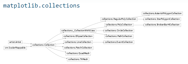
    path = axes[1, 1].collections[0].get_paths()[0]
    patch = mpl.patches.PathPatch(path, transform=axes[1, 1].transData)
    im.set_clip_path(patch)

    # RGB
    sns.kdeplot(mandrill_rgb[:, :, 0].ravel(), bw_adjust=0.5, cut=1, fill=True, alpha=0, color="red", label="R", ax=axes[1, 2])
    sns.kdeplot(mandrill_rgb[:, :, 1].ravel(), bw_adjust=0.5, cut=1, fill=True, alpha=0, color="green", label="G", ax=axes[1, 2])
    sns.kdeplot(mandrill_rgb[:, :, 2].ravel(), bw_adjust=0.5, cut=1, fill=True, alpha=0, color="blue", label="B", ax=axes[1, 2])
    for i, color in enumerate(["red", "green", "blue"]):
    im = axes[1, 2].imshow(np.vstack([x, x]), cmap=f"{color.capitalize()}s_r",
    aspect="auto", extent=[*axes[1, 2].get_xlim(), *axes[1, 2].get_ylim()])
    path = axes[1, 2].collections[i].get_paths()[0]
    patch = mpl.patches.PathPatch(path, transform=axes[1, 2].transData)
    im.set_clip_path(patch)
    axes[1, 2].set_ylim(top=axes[1, 2].get_ylim()[1] * 1.4)
    axes[1, 2].legend(ncol=3, fontsize=9)

    # alpha
    axes[0, -1].imshow(ruler, zorder=-1, cmap="gist_gray")
    sns.kdeplot(mandrill_alpha[:, :, 0].ravel(), bw_adjust=0.5, cut=1, fill=True, alpha=0, color="red", label="R", ax=axes[1, 3])
    sns.kdeplot(mandrill_alpha[:, :, 1].ravel(), bw_adjust=0.5, cut=1, fill=True, alpha=0, color="green", label="G", ax=axes[1, 3])
    sns.kdeplot(mandrill_alpha[:, :, 2].ravel(), bw_adjust=0.5, cut=1, fill=True, alpha=0, color="blue", label="B", ax=axes[1, 3])
    sns.kdeplot(mandrill_alpha[:, :, 3].ravel(), bw_adjust=0.5, cut=1, fill=True, alpha=0, color="k", label="alpha", ax=axes[1, 3])
    for i, color in enumerate(["red", "green", "blue"]):
    im = axes[1, 3].imshow(np.vstack([x, x]), cmap=f"{color.capitalize()}s_r",
    aspect="auto", extent=[*axes[1, 3].get_xlim(), *axes[1, 3].get_ylim()])
    path = axes[1, 3].collections[i].get_paths()[0]
    patch = mpl.patches.PathPatch(path, transform=axes[1, 3].transData)
    im.set_clip_path(patch)
    axes[1, 3].set_ylim(top=axes[1, 3].get_ylim()[1] * 1.4)
    handles, labels = axes[1, 3].get_legend_handles_labels()
    axes[1, 3].legend(handles=handles[-1:], labels=labels[-1:], fontsize=9)

    for ax in axes[1]:
    ax.set_xlim(-0.1, 1.1)
    ax.set_yticklabels([])
    ax.set_xlabel('intensity', fontsize=12, labelpad=8)
    ax.set_ylabel('')


    fig.tight_layout()


도움이 되셨나요? 카페인을 투입하시면 다음 포스팅으로 변환됩니다

Share