- 정지된 그림으로는 볼 수 없는 것들이 있습니다.
- 시간에 따른 변화나 입체 도형의 뒷면이 그것입니다.
- 애니메이션을 활용해 이를 보완합니다.
1. Matplotlib animation
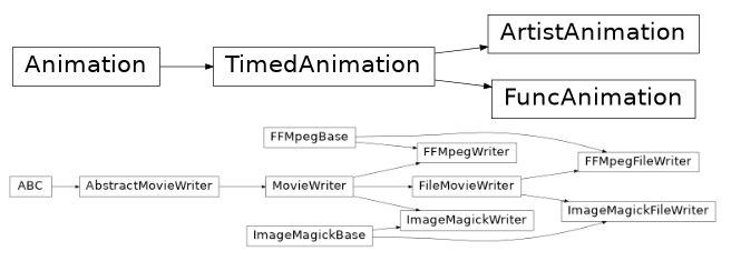
- Matplotlib에서 사용할 수 있는 애니메이션은 두 가지가 있습니다.
- Artist 객체 변화를 저장하는
ArtistAnimation, - Figure 전체의 변화를 저장하는
FuncAnimation이 그 것입니다.
1.1. base figure
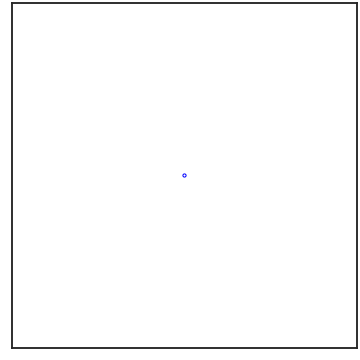
- 간단한 그림을 그려서 애니메이션으로 만듭니다.
- 가운데 동그라미를 하나 그리고, 이 동그라미가 점점 커지는 모습을 구현합니다.
- 기본 명령어를 사용해 화면 한가운데 동그라미를 그립니다.
1 | # 기본 설정 |
- 객체 지향 방식을 사용해 이 객체의 크기를 바꾸겠습니다.
- circle이라는 이름으로 저장한 marker 하나는 collections로 다루어집니다.
.set_sizes()에 list 형태로 새로운 size를 전달하여 크기를 변경합니다.- marker가 하나밖에 없으므로 원소가 하나뿐인 list를 입력합니다.
- 이를
update()라는 이름의 함수로 만들어 적용합니다.
1 | # marker 크기 변경 함수 |
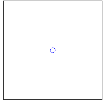
- 화면 가운데 있는 원이 커졌습니다.
- 이제 연속적으로 적용하고 .gif 파일로 적용하면 애니메이션이 됩니다.
1.2. FuncAnimation
- frame마다 변하는 Figure 차례로 저장해 애니메이션으로 만듭니다.
- Figure 객체에 위에서 만든
update()같은 함수를 연속적으로 적용합니다. - 이 때 사용하는 함수가
FuncAnimation이고, Figure 객체, 함수와 함께frames에 총 프레임을 넣고, intervals에 frame 사이 시간 간격을 ms단위로 입력합니다.- 위 두 코드 뒤에
FuncAnimation한 줄을 추가하고,.save()로 파일로 저장합니다.
1 | from matplotlib.animation import FuncAnimation |

1.3. ArtistAnimation
- 조금 다른 방식으로 artist 객체의 변화를 저장해 animation을 만들 수 있습니다.
- Artist에 변화를 준 내용을 list로 저장해서
ArtistAnimation()에 전달하는 방식입니다. FuncAnimation()에는 함수를 전달했던 것과 다른 방식입니다.- 함수로 표현하기 어려운 급격한 변화도 담을 수 있지만 리스트가 담길 메모리는 다소 부담이 됩니다.
1 | from matplotlib.animation import ArtistAnimation |

- 같은 애니메이션을 구현했습니다.
2. 3D 도형 시각화 적용
2.1. z axis 주변 회전
- 원래의 목적인 3D 도형의 뒷면을 보여주는 시각화를 수행합니다.
- Matplotlib 공식 홈페이지에 있는 구조를 가져와 다른 방식으로 그립니다.
Axes.contourf()를 3D Axes에 표현해보고,- 다른 공간에는
Axes.plot_surface()와 함께 아래 면을 사용합니다.
1 | # 2D mesh grid |
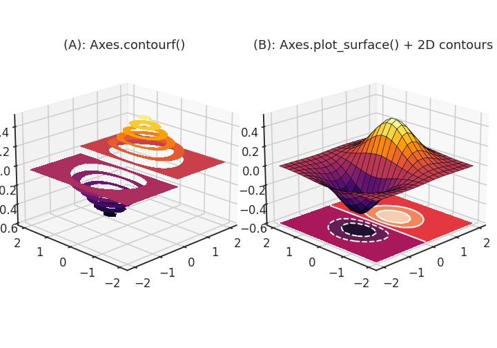
- 제법 멋진 그림이 그려졌지만 뒷부분이 보이지 않습니다.
- 한 frame에 2도씩, 두 그림 모두 회전시킵니다. 180 frame을 적용해 한바퀴를 돌립니다.
1 | # animation frame마다 적용되는 변화 |
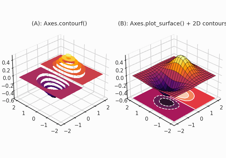
- 빙글빙글 돌아가는 모습이 표현됩니다.
2.2. 3D 회전
-
이번에는 조금 더 자유롭게 회전시켜보겠습니다.
-
Axes.view_init()에 들어가는 두 개의 인자,elev와azim에 랜덤으로 만든 array를 입력하면 됩니다. -
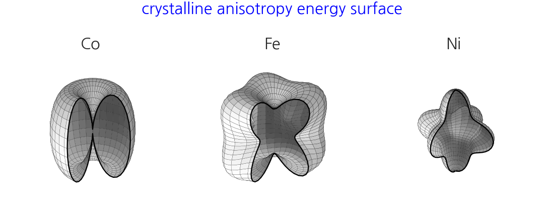
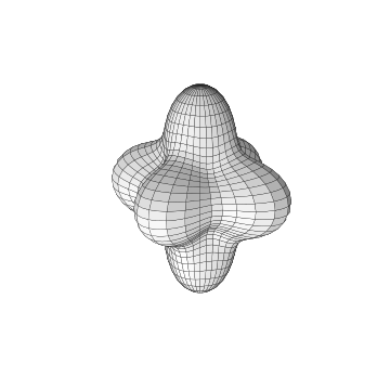
돌려보는 재미가 있는 3D 객체를 생성합니다. 오른쪽 Ni 그림을 사용합니다.
-
과거 글에 있는 그림을 사용합니다.
-
핵심 코드만 가져옵니다.
-
잘려진 부분 없이 온전한 모습으로 그립니다.
1 | from itertools import product |
elev와azim을 미리 array로 만들어 두고,- frame_number를 index로 사용해 하나씩 꺼내는 함수를 만듭니다.
- 그리고,
FuncAnimation()에서 이들을 호출해 애니메이션을 생성합니다.
1 | frames = 360 |
- 3차원 공간을 자유롭게 회전하는 영상이 되었습니다.
