-
PyTorch는 현재 가장 인기있는 딥러닝 라이브러리 중 하나입니다.
-
학습 세부 사항을 지정하기 위해 Callback으로 다양한 기능을 지원합니다.
-
skorch는 PyTorch를 scikit-learn과 함께 사용할 수 있게 해 줍니다.
-
skorch도 PyTorch callback을 이용할 수 있습니다.
-
글이 길어 세 개로 나눕니다.
-
세 번째로, skorch를 사용해 ML Pipeline을 완성합니다.
-
여러 callback으로 자세한 설정을 반영합니다.
3.2. skorch
- Colab에는 skorch가 기본으로 설치되어 있지 않습니다.
- 간단한 명령으로 skorch를 설치합니다.
1 | !pip install skorch |
3.2.1. preprocessor 포함 pipeline 작성
-
앞에서 만든
get_preprocessor()함수는 전처리 Pipeline을 출력합니다. -
Pipeline을 연장해 이 뒤에 PyTorch로 만든 Neural Network를 덧붙입니다.
-
우리가 푸는 문제는 펭귄의 체중을 구하는 regression문제입니다.
-
skorch에서 제공하는
NeuralNetRegressor()로 PyTorch 신경망을 감쌉니다. -
loss function, optimizer 등은
NeuralNetRegressor()안에criterion,optimizer등의 매개변수를 사용해 입력합니다. -
optimizer=optim.Adam으로 Adam을 선택했습니다. -
PyTorch에서 Adam()안에 들어가던 매개변수
lr=1e-3은optimizer__lr=1e-3으로 바뀌어 들어갑니다.
1 | import skorch |
- 실행 결과 : 너무 길어서 out of memory 오류가 뜰 수 있습니다. 침착하게 새로 고침을 누르시면 됩니다.
- 또는,
verbose=1을verbose=0으로 바꾸시는 것도 방법입니다.
1 | ... (생략) ... |
-
학습이
model.fit()으로 잘 됩니다. -
NeuralNetRegressor로 한 번 감싼 것 만으로 scikit-learn API를 사용할 수 있게 되었습니다. -
X_train대신 전처리를 거친X_train_np를 입력했습니다. -
y_train대신으로는y_train.astype(np.float32).values.reshape(-1, 1)이 들어갔습니다. -
pandas Series에서 데이터 타입을 바꾸고, 값을 추출해서, shape을 바꾼 것입니다.
-
예측도
model.forward()대신model.predict()로 진행합니다.
1 | # prediction |

3.2.2. ML pipeline 작성
skorch: skorch.callbacks.InputShapeSetter
stackoverflow: How to pass input dim from fit method to skorch wrapper?
-
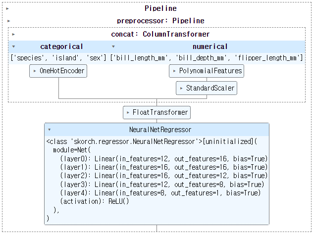
앞에서 만든 전처리기,
get_preprocessor()를 포함하는 Pipeline을 만듭니다. -
method매개변수로 neural network 뿐 아니라 linear regression, random forest를 선택할 수 있게 합니다. -
Neural network는 이들 방법들과 달리 input dimension이 중요합니다.
-
신경망 구조를 만들 때 필요한 변수이기 때문입니다.
-
callback은 여러 설정을 지정할 수 있는 방법입니다.
InputShapeSetter를 callback에 기본값으로 박아 넣습니다. -
그 외에 여러 keyword arguments를 입력할 수 있도록
**kwargs를NeuralNetRegressor()에 추가합니다.
1 | # machine learning models |
- 이제
get_model()을 사용해 ML pipeline을 제작할 수 있습니다. method에 입력하는 값에 따라 선형 회귀, 앙상블 트리, 신경망을 선택할 수 있습니다.
1 | model = get_model("nn", max_epochs=epochs, verbose=1, criterion=RMSELoss, optimizer=optim.Adam, optimizer__lr = 1e-3) |
- 웬만한 매개변수는 모두
NeuralNetRegressor()에 들어갑니다. - 어떤 매개변수들이 있는지 출력해서 확인합니다.
1 | model["ml"].get_params() |
- 실행 결과
1 | {'_kwargs': {'optimizer__lr': 0.001}, |
3.2.3. train and validate (self)
- X_train과 y_train만 사용해서 학습시킵니다.
1 | model.fit(X_train, y_train.values.reshape(-1, 1).astype(np.float32)) |
- 실행 결과
1 | Re-initializing module because the following parameters were re-set: module__ninput. |
-
validation set을 입력하지 않았음에도 valid_loss가 출력됩니다.
-
train data의 20%를 validation set으로 따로 떼어 놓기 때문입니다.
-
맨 처음 전체 데이터의 60%만 train set으로 지정했습니다.
-
여기서 다시 80%만 학습에 투입되었으니 총 48%. 반도 안되는 데이터로 학습한 셈입니다.
-
train_split=None을 입력하면 모든 데이터를 다 학습에 투입하지만 validation 결과가 출력되지 않습니다. -
learning curve는 신경망에서
.history속성을 추출해 확인할 수 있습니다.
1 | history = model["ml"].history |
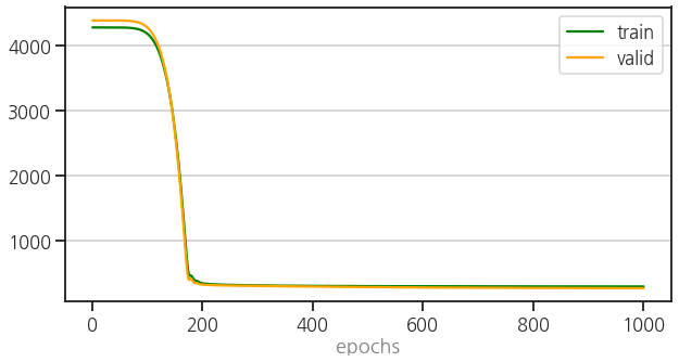
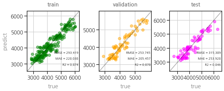
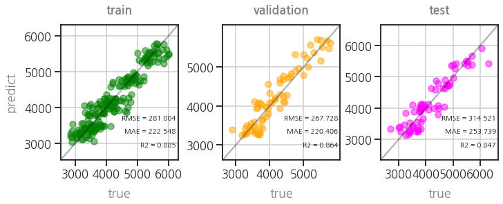
- 학습도 정상적으로 이루어졌습니다.
1 | plot_parity3(model) |
3.2.4. train and validate (predefined validation set)
- 먼저 준비한 validation set을 사용하려면
train_split에 validation set을 입력합니다. - validation set은 skorch의
Dataset을 사용해 만듭니다. - 내친 김에 y data도 ML Pipeline에 만들기 좋은 형태, 즉 float32, (-1, 1) shape으로 변경해서 모아놓습니다.
1 | from skorch.dataset import Dataset |
- 실행 결과
1 | Re-initializing module because the following parameters were re-set: module__ninput. |
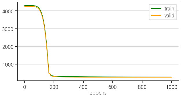
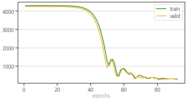
- learning curve를 확인합니다.
- 여기서 얻은 learning curve를 reference로 사용하겠습니다.
1 | history = model["ml"].history |
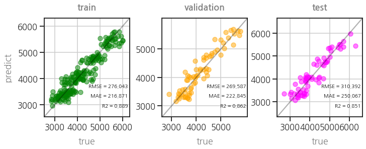
- parity plot도 확인합니다.
1 | plot_parity3(model) |
3.2.5. learning rate scheduler
skorch: Learning rate schedulers
Pega Devlog: Fast.ai의 fit_one_cycle 방법론 이해
- callbacks에 learning late scheduler를 추가해 learning rate를 조정할 수 있습니다.
- input dimension 조정을 위해 callbacks 기본값으로 InputShapeSetter()가 들어가 있습니다.
- 이를 삭제하지 않도록 유의하면서 learning rate scheduler를 추가합니다.
1 | from skorch.callbacks import LRScheduler |
- 학습 과정은 생략하고 learning curve를 비교해서 봅니다.
1 | ax = plot_epoch(train_loss_0, valid_loss_0) |
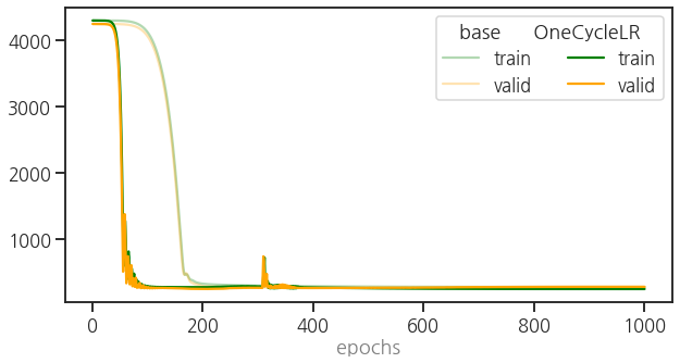
- learning rate scheduler가 적용되어 학습 양상이 바뀌었습니다.
- parity plot도 여전히 좋습니다.
1 | plot_parity3(model) |

3.2.6. early stopping
- 불필요하게 학습을 길게 하는 경향을 줄이고자 early stopping을 적용합니다.
EarlyStopping()을 callbacks에 추가하고 기준을 설정합니다.- valid_loss가 20번 줄어들지 않으면 학습을 중단하도록
monitor="valid_loss",patience=20을 설정했습니다.
1 | from skorch.callbacks import EarlyStopping |
- learning curve를 비교합니다.
1 | ax = plot_epoch(train_loss_0, valid_loss_0) |
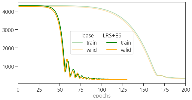
- parity plot도 정상적입니다.
1 | plot_parity3(model) |

3.2.7. Saving and Loading (manual)
- 모델 파라미터를 pickle 형식으로 저장하고 불러올 수 있습니다.
1 | # save parameters |
- 모델을 새로 만들면 paramter를 불러오기 전에 초기화하는 과정이 필요합니다.
.initialize()를 사용합니다.
1 | # load parameters |
- 새로 만든 모델에 parameter를 불러와서 적용합니다.
- 단, 신경망 parameter에만 해당하는 상황이므로 preprocessor는 기존 모델의 preprocessor를 사용합니다.
1 | # check reproducibility |

- 학습을 하지 않았음에도 parity plot이 똑같이 재현되었습니다.
3.2.8. Saving and Loading (callbacks)
- callback을 이용하면 valid loss가 줄어들때마다 저장할 수 있습니다.
- valid loss가 줄어들때마다 저장하는
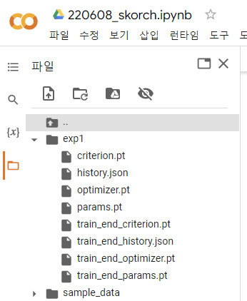
cp와 epoch마다 저장하는train_end_cp를 동시에 지정합니다. exp1폴더를 만들어 여기에 함께 저장하도록 합니다.
1 | from skorch.callbacks import Checkpoint, TrainEndCheckpoint |
- 실행 결과
1 | Re-initializing module because the following parameters were re-set: module__ninput. |
-
cp라는 열이 하나 생겼고, 여기 +가 붙은 곳들이 있습니다.
-
valid_loss가 기존 기록보다 작아진 지점입니다.
-
History도 파일에서 불러와서 그립니다.
-
부를 때는
skorch.history.History를 사용합니다. -
세 개의 learning curve를 겹쳐 그리느라 코드가 다소 복잡해졌습니다.
1 | from skorch.history import History |
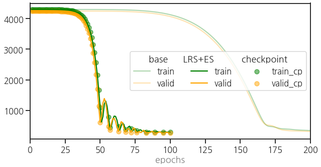
- 희미하게 그려진 것은 skorch에 validation set을 사용한 base line입니다.
- 그리고 Learning Rate Scheduler와 Early Stopping을 적용한 것을 LRS + ES로 표기했습니다.
- 앞에서와 같이 학습이 훨씬 빨리 끝났습니다.
- 그리고 이 중 checkpoint가 적용된 것을 scatter plot으로 표현했습니다.
- one-cycle-fit의 영향으로 learning curve가 요동치는 와중에서도 train과 valid에서 단조 감소하는 모습만이 기록되었습니다.
3.2.9. valid loss가 가장 적었던 checkpoint 불러서 learning rate 낮추기
-
각 checkpoint에서는 history 외에도 criterion, optimizer, parameter 등의 상태를 저장합니다.
-
Colab 왼쪽의 폴더 모양을 클릭해 저장한 파일을 확인하면 볼 수 있습니다.
-
학습이 과하게 진행되어 overfitting이 되면 지나가버린 과거의 최적점이 아쉽습니다.
-
지나친 최적점을 불러와서 훨씬 낮은 learning rate로 살살 학습시키면 더 좋을 것 같습니다.
-
이 때 skorch에서 제공하는 LoadInitState를 사용할 수 있습니다.
-
cp = Checkpoint()로 저장된 위치를 지정하고, -
load_state = LoadInitState(cp)로 불러와 상태를 불러옵니다. -
마지막으로
callbacks에cp와load_state를 추가합니다.
1 | from skorch.callbacks import LoadInitState |
3.2.10. Saving and Loading (model itself)
- 모델 전체를 저장할 때는 pickle을 권장하고 있습니다.
pickle.dump()와pickle.load()를 사용해 모델을 읽고 씁니다.
1 | # saving |
- 저장한 모델을 불러오면서 이름을 model_pkl로 바꿨습니다.
- 이 모델의 parity plot을 그려서 잘 저장되었고 불러졌는지 확인합니다.
1 | # check reproducibility |
- 추가 학습 없이도 원래의 성능이 확인되었습니다.
4. 정리 : skorch ML pipeline
-
이제까지 세 편의 글에 걸쳐 데이터를 정리한 후,
-
scikit-learn preprocessor를 만들고,
-
PyTorch neural network를 구축한 후,
-
skorch로 이들을 엮은 뒤 callbacks로 여러 옵션을 뿌렸습니다.
-
최종적으로 사용한 코드가 여기 저기 흩뿌려져 있어 활용이 어려울 듯도 싶습니다.
-
skorch ML pipeline 코드를 아래에 정리합니다.
-
목적은 Ctrl+C/V와 약간의 수정으로 사용하는 것입니다.
4.1. skorch ML pipeline
- scikit-learn preprocessor
1 | # preprocessors |
- PyTorch Neural Network
1 | import torch |
- skorch ML Pipeline
1 | # machine learning models |
4.2. Visualizations
- learning curve
1 | def plot_epoch(history=None, loss_trains=None, loss_vals=None, ax=None): |
- parity plots
1 | def plot_parity3(model, target=["train", "val", "test"], figsize=(10, 4), |
4.3. test run
- 정의한 함수들로 예제를 돌려봅니다.
1 | # predefined validation set |
- 실행 결과
1 | Re-initializing module because the following parameters were re-set: module__ninput. |

- 잘 돌아갑니다. :)
- 전체를 실행해볼 수 있는 코드는 여기 있습니다: Notebook
