Contributor
김승욱님, dane님
References
wikipedia: Stratified Sampling
When should you choose Stratified sampling over random sampling?
핸즈온 머신러닝 (2판)
핸즈온 머신러닝 (2판): 2장 - 머신러닝 프로젝트 처음부터 끝까지 notebook
1. Introduction to Stratified Sampling
- 데이터 분석을 위해 일부의 데이터를 가져오는 것을 추출(sampling)이라 합니다.
- 인위적인 편향을 방지하기 위해 아무렇게나 가져오는 임의추출(random sampling)을 사용합니다.
- 그러나 임의추출은 데이터의 비율을 반영하지 못한다는 단점이 있어, 층화추출(stratified sampling)이 권장됩니다.
- 적절한 층화추출은 임의추출보다 항상 좋다는 것이 증명되어 있다고 합니다.
1.1. 층화추출 적용 과정
- 층화추출을 적용하려면 여러 기법을 함께 사용해야 합니다.
(1). 층화추출은 범주형(categorical) 데이터에 적용하는 기법입니다.
- 수치형(numerical) 데이터는 먼저 계층화(stratification)를 해야 합니다.
- 계층화는 이산화(discritization), 양자화(quantization)등으로도 불리는데, 연속적으로 이어진 데이터를 사전에 정의된 구간으로 분할하는 과정입니다.
(2). 범주형 데이터는 인코딩(encoding)을 해야 할 수 있습니다.
- 데이터 연산시 문자열(string)로 되어 있는 데이터는 숫자열 변환이 필요합니다.
- 훈련 세트에 없는 항목이 테스트 세트에 들어올 경우 오류를 내고 중지를 하거나 (오류를 감안하고) 무시하고 진행해야 하는데, 그럴려면 훈련 세트의 인코딩 정보를 기억하고 테스트 세트에 적용할 장치가 필요합니다.
- 기계적으로
pandas.get_dummies()를 훈련 세트, 테스트 세트에 따로 적용하면 안 된다는 말씀입니다.
- 훈련 데이터 기준으로 전처리기(preprocessor)를 세팅하고 머신러닝 모델을 학습해야 합니다.
1.2. 층화추출 지원 함수
-
scikit-learn은 지정된 변수에 대한 층화추출을 여러 방식으로 지원합니다.StratifiedShuffleSplit(): 층화추출 후 index를 반환합니다.StratifiedKFold(): K Fold를 만든 후 index를 반환합니다.train_test_split(): 비율대로 분할한 데이터셋을 반환합니다.
-
핸즈온 머신러닝의 캘리포니아 주택 가격 예제를 통해 Stratified Sampling 과 Random Sampling을 비교해보겠습니다.
- 핸즈온 머신러닝에서는
StratifiedShuffleSplit()을 사용했습니다. - 그러나 사용해보면 아시겠지만
train_test_split()이 더 편합니다. - 왜 굳이
StratifiedShuffleSplit을 쓴걸까 궁금했는데 이런 히스토리가 있었네요.
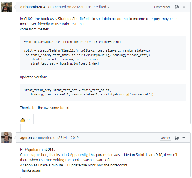
- 핸즈온 머신러닝에서는
2. Data Load and Sampling
- 글이 지나치게 길어지는 것을 막고자 데이터 로드 부분은 생갹하겠습니다.
- 전체 코드는 여기에서 받아보실 수 있습니다.
- 핸즈온 책의 역자, 박해선님이 올려주신 colab 코드를 보셔도 좋습니다.
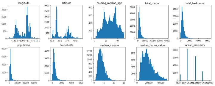
2.1. Data Load
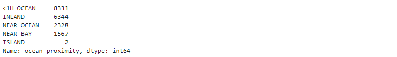
- 원본 데이터에서 이상치에 해당하는 부분을 제거한 뒤의 비율은 다음과 같습니다.
1 | housing_r = housing.copy() |
1 | housing_r['ocean_proximity'].value_counts() |
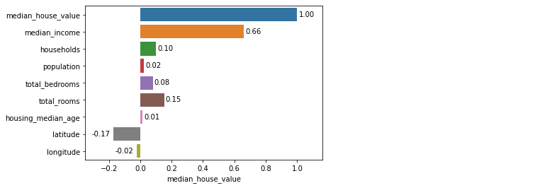
- target 변수인
median_house_value와 가장 연관성이 높은 변수는median_income입니다. - 아래
fig, ax = plt.subplots()하단 대신sns.heatmap(cor, annot=True)한방이면 더 쉽게 변수별 연관성을 볼 수 있지만 bar plot으로 표현해 보겠습니다.
1 | columns = list(housing_r) |
2.2. Data Sampling
- 훈련/테스트 세트를 나눌 때, 주요 변수인
median_income에 층화추출을 적용하겠습니다. - 그리고
ocean_proximity에도 함께 적용해서 층화추출 변수 추가 효과를 보겠습니다.
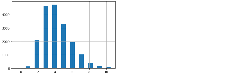
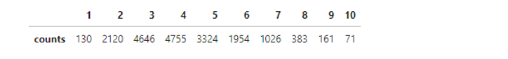
2.2.1. Data Quantization: ‘median_income’
- 층화추출 적용에 앞서 데이터 계층화를 수행합니다.
1 | bins = [0, 1, 2, 3, 4, 5, 6, 7, 8, 9, np.inf] |
2.2.2. Data Sampling: Random and Stratified Sampling
- 먼저 임의추출을 수행해 봅니다.
1 | from sklearn.model_selection import train_test_split |
- 이번엔 층화추출을 수행합니다.
train_test_split()에stratify=변수명을 넣어주면 됩니다.
1 | train_strat, test_strat = train_test_split(housing_r, test_size=0.3, |
- random seed를 고정해서 반복수행에도 동일한 결과가 나오도록 하였습니다.
- 추출 결과를 비교해 보겠습니다.
1 | def income_cat_proportions(housing_r): |
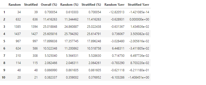
- random state가 동일함에도 불구하고 두 결과가 살짝 다릅니다.
- 층화추출이 전체 데이터의 비율을 더 잘 반영하고 있습니다.
- 아까 만든 income_cat 데이터는 용도를 다 했으니 지웁니다.
1 | train_random = train_random.drop("income_cat", axis=1) |
- 입력 인자(X)와 목표값(Y)을 분리합니다.
1 | Y_train_random = train_random['median_house_value'] |
- 많은 코드에서 전체 데이터를 X와 Y로 먼저 분리한 후
train_test_split()을 이용해 훈련 세트와 테스트 세트를 만들지만 층화추출을 적용하려면 훈련/테스트 세트를 먼저 분할해야 합니다. - 이제 이 데이터를 이용한 머신러닝의 결과를 비교해 보겠습니다.
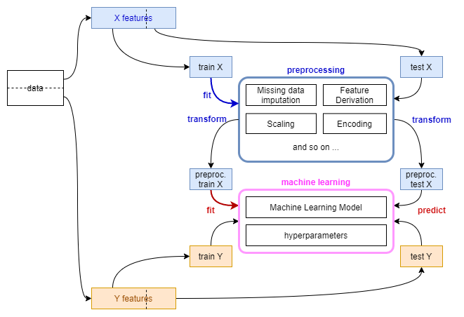
2.3. Preprocessing Pipeline
- 앞에서 범주형 변수를 처리하기 위해 인코딩을 한다고 말씀 드렸습니다.
- 훈련 세트에 적용된 기준을 저장했다가 테스트 세트에 적용해야 한다고도 말씀 드렸습니다.
- 이럴 때 사용하기 좋은 것이
Pipeline()입니다. - 자세한 내용은 여기에 맡기고 간단하게만 언급합니다.
- 수치형 데이터의 결측치를 median으로 메웁니다.
- 인자간 연산을 통해 파생변수를 추가합니다.
- 수치데이터에 standard scaling을 적용합니다.
- 범주형 데이터에 원핫 인코딩을 적용합니다.
handle_unknown='ignore': 테스트 세트에서 새로운 클래스를 만날 때 무시하라는 의미입니다.
기본값인 'error’는 오류를 내면서 중지하라는 의미입니다.drop=None: [0, 0, …, 0]으로 표기될 테스트 클래스의 새로운 클래스가 기존 클래스와 혼동되지 않도록 조치를 취합니다.
1 | num_pipeline = Pipeline([("imputer", SimpleImputer(strategy="median")), |
fit_transform()으로 훈련 데이터를 이용한 인코더 설정fit()과 변수 변환transform()을 동시에 합니다.- 테스트 데이터는 훈련 데이터 기준으로 변환해야 하므로
fit()이 없는transform()만 해야 합니다.
1 | pipeline_random = deepcopy(full_pipeline) |
3. Machine Learning
- 본 글에선 머신러닝 모델링은 최소한의 노력으로 수행하겠습니다.
- 모델은 hyperparameter를 고정한
RandomForestRegressor를, 평가 방식은 root mean squared error를 사용하겠습니다.
1 | from sklearn.ensemble import RandomForestRegressor |
3.1. Overall data
- 임의추출 방식
1 | rf_random = RandomForestRegressor(n_estimators=30, max_features=8, random_state=42) |
44628.384490024335
- 층화추출 방식
1 | rf_strat = RandomForestRegressor(n_estimators=30, max_features=8, random_state=42) |
44743.58037848807
-
층화추출 방식의 에러가 조금 더 적습니다.
-
그림으로 비교해 보면 어떨까요?
-
코드는 생략합니다. 전체 코드를 참고해주세요.
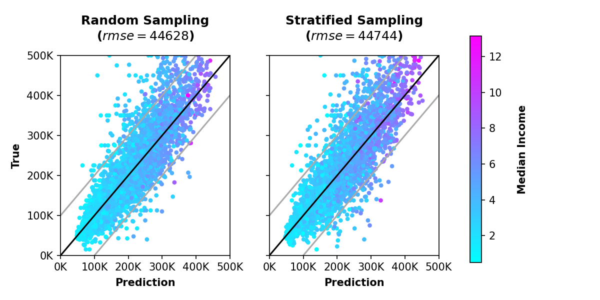
-
차이가 있는 듯 없는 듯 합니다.
-
앞서 소득을 10개의 구간으로 세분화했으므로, 구간별 예측력을 살펴봅시다.
3.2. data by bins
- 소득(
median_income) 구간별 예측력을 분석해 보겠습니다. - 구간별 데이터를
DataFrame의 index로 접근해야 하니 리셋부터 해줍니다.
1 | X_test_random.reset_index(drop=True, inplace=True) |
- 그리고 구간별로 데이터를 따로따로 모아 분리해 줍니다.
1 | Y_pred_random_bin = [] |
- seaborn에서 bar plot을 그릴 수 있도록 데이터프레임으로 묶어줍니다.
1 | df_RMSE_random = pd.DataFrame({'RMSE': RMSE_random, |
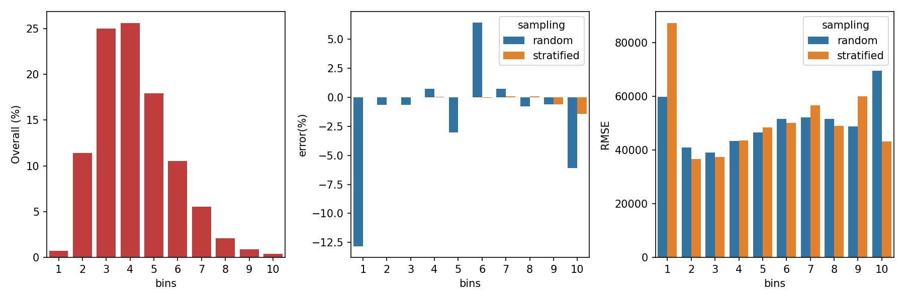
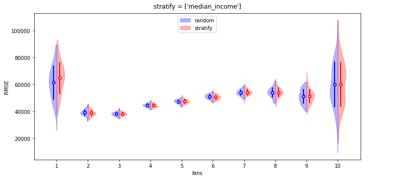
- 가운데 그림에서 앞서 보았던, 층화추출의 적은 추출 오차율이 한눈에 보입니다.
- 그러나 무색하게도 맨 오른쪽 그림을 보면, 첫번째와 9번째 구간에서 층화추출의 오차가 매우 큽니다. 층화추출 결과가 눈에 띄게 좋은 구간은 10번째 구간 뿐이고 나머지는 비슷비슷하네요.
4. Statistical Analysis
-
편한 임의추출 방식을 놔두고 층화추출을 했는데 에러가 커지니 속이 상합니다.
-
혹시
train_test_split()에 사용된random_state에 따라 왔다갔다 하는 건 아닐까요? 층화추출이 전체 데이터의 비율을 더 잘 반영하는 것은 자명하니, 임의추출에서 어쩌다 무의미한 높은 성능이 나온 것은 아닐까요? -
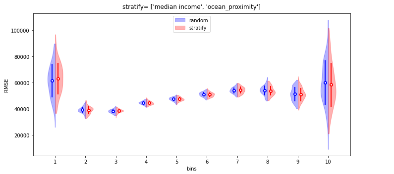
random_state만 바꿔가면서 100번 돌려서, 층화추출을 1개 변수(median_income)와 2개 변수(median_income,ocean_proximity)에 적용한 경우를 비교해 봤습니다. -
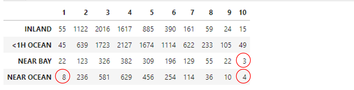
여기, 층화추출시 한 가지 주의사항이 더 붙습니다.
-
변수 하나만 층화추출할 때는 그래도 괜찮은데 :
median_income
-
변수 두 개로 층화추출을 실시하면 and 조건으로 인해 원소가 매우 작은 집합이 생깁니다.
-
이러면
train_test_split()같은 scikit-learn 제공 분할 메소드에서 에러를 낼 수 있습니다. -
원소가 최소 두 개는 되어야 한다면서 프로그램이 다운되어 버립니다.
4.1. Visualization
- violin plot을 split 할 때 seaborn을 사용하면 편리하지만 numpy 버전이 14 이상일 경우 작동되지 않는 버그가 발생하기도 합니다.
- 다소 성가시지만 matplotlib을 이용해 수동으로 구현했습니다.
1 | import matplotlib.patches as mpatches |
4.2. Test on Variances and Means
- 육안으로는 차이를 구분하기 힘듭니다만 임의추출과 층화추출간 평균과 분산이 같은지 확인해 보겠습니다.
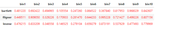
- 분산 비교는
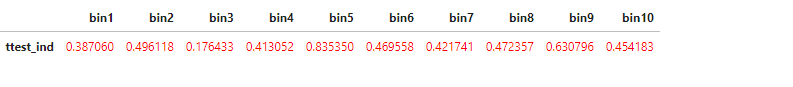
scipy.stats에 포함된 3가지의 등분산 검정-bartlett(),fligner(),levene()을, 평균 비교는 T 검정 중 독립표본 T 검정-ttest_inds()을 이용하겠습니다. - p-value가 0.05 미만일 경우 분산 또는 평균이 다르다고 가정하여, 0.05를 기준으로 DataFrame의 글자 색상을 다르게 넣어주도록 했습니다. 동일하면 빨간색, 다르면 파란색.
1 | import scipy.stats as stats |
4.2.1. 1변수 층화추출
-
등분산 검정결과
-
T 검정 결과

-
평균과 분산 모두 임의추출과 층화추출이 동일하다는 결론입니다.
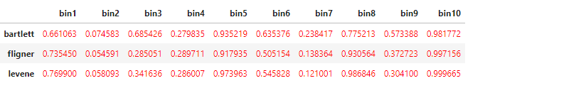
4.2.2. 2변수 층화추출
-
등분산 검정결과
-
T 검정 결과
-
마찬가지로 추출 방식에 무관하다는 결론입니다.
5. Conclusion
-
결과적으로, 본 예제에서는 임의추출과 층화추출간 유의차를 발견하기 힘듭니다.
-
때로는 임의추출과 유의차가 없다는 것 또한 배움이겠죠. :)
-
비슷한 비교를 한 다른 분의 결과에서도 층화추출의 예측력이 증대되지는 않았다는 결과가 있으나, 재밌게도 여기서는 층화추출의 경우 훈련과 학습에 소요되는 시간이 줄어들었다고 합니다.
-
층화추출은 높은 점수보다는 결과에 대한 신뢰성을 위해 사용하는 방법입니다.
-
임의추출도 데이터 비율을 상당히 반영하기 때문에 신뢰성이 없다고 할 수 없지만 층화추출만큼 체계적이라 말하기 힘듭니다.
-
임의추출에서 층화추출과 유사한 결과를 얻었다 하더라도, 직접적으로 비교를 하지 않는 이상 개선의 여지가 있어 보이는 우연으로 느껴질 수 밖에요.
-
파이프라인에 익숙하지 않으신 분이라면 층화추출 과정이 번거롭다고 느껴질 수 있겠지만 임의추출이라고 계층화 정도가 생략될 뿐, 과정이 달라지지는 않습니다.
-
테스트세트를 가린 채 훈련 세트의 데이터 분포 기준으로 테스트 세트에도 동일한 기준의 전처리를 해야 하고, 그러자면 파이프라인만큼 효과적인 것이 없기에 파이프라인 구축은 습관을 들여야 합니다.
