Seaborn with Matplotlib (1)

1. seaborn + matplotlib

• seaborn을 matplotlib과 섞어쓰는 방법입니다.
• 4부 중 첫 번째 시간입니다.
• seaborn 함수 중 matplotlib axes를 반환하는 함수들에 관한 내용입니다.

seaborn API

• seaborn은 matplotlib을 쉽고 아름답게 쓰고자 만들어졌습니다.

  • 따라서 seaborn의 결과물은 당연히 matplotlib의 결과물입니다.
  • 그러나 간혹 seaborn이 그린 그림의 폰트, 색상에 접근이 되지 않아 난처합니다.
  • seaborn의 구조를 잘 이해하지 못하면 해결도 어렵습니다.

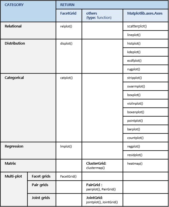
• v0.11 기준으로 seaborn에는 다음 함수들이 있습니다.
  
  

• matplotlib의 출력물은 figure와 axes만을 반환합니다.
  • seaborn의 명령어 중 axes를 반환하는 것들은 matplotlib과 섞어 쓰기 좋습니다.
  • 먼저 matplotlib의 객체 지향object oriented interface를 사용해서 그림의 틀을 만든 뒤,
  • 특정 axes에 seaborn을 삽입하면 됩니다.
  • 결론적으로, 하고 싶은 거 다 됩니다.

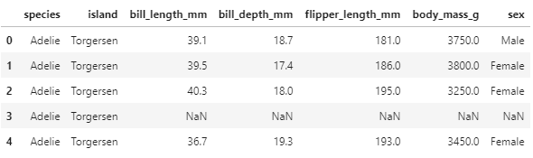
1.1. Load data

• 예제로 사용할 펭귄 데이터를 불러옵니다.
• seaborn에 내장되어 있습니다.

  import pandas as pd
  import matplotlib.pyplot as plt
  import seaborn as sns
  
  penguins = sns.load_dataset("penguins")
  penguins.head()

  

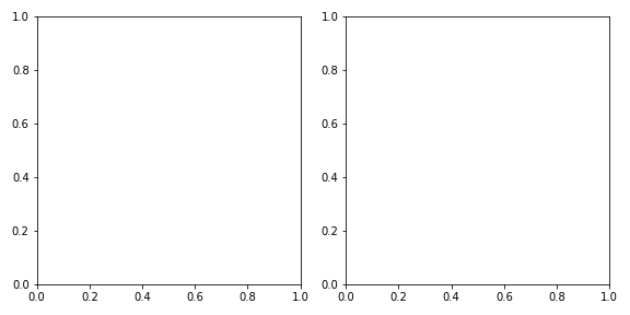
1.2. figure and axes

• matplotlib으로 도화지figure를 깔고 축공간axes를 만듭니다.
• 1 x 2 축공간을 구성합니다.

  fig, axes = plt.subplots(ncols=2, figsize=(8,4))
  
  fig.tight_layout()

  

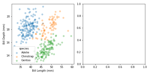
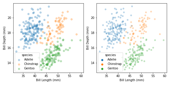
1.3. plot with matplotlib

• matplotlib 기능을 이용해서 산점도를 그립니다.
  • x축은 부리 길이 bill length
  • y축은 부리 위 아래 두께 bill depth
  • 색상은 종species로 합니다.
    Adelie, Chinstrap, Gentoo이 있습니다.

• 두 축공간 중 왼쪽에만 그립니다.

  fig, axes = plt.subplots(ncols=2, figsize=(8, 4))
  
  species_u = penguins["species"].unique()
  
  # plot 0 : matplotlib
  for i, s in enumerate(species_u):
      axes[0].scatter(penguins["bill_length_mm"].loc[penguins["species"]==s],
                     penguins["bill_depth_mm"].loc[penguins["species"]==s],
                     c=f"C{i}", label=s, alpha=0.3
                    )
  axes[0].legend(species_u, title="species")
  axes[0].set_xlabel("Bill Length (mm)")
  axes[0].set_ylabel("Bill Depth (mm)")
  
  fig.tight_layout()

  

1.4. plot with seaborn

seaborn scatterplot

• 이번엔 같은 plot을 seaborn으로 그려봅니다.
• 위 코드에 아래 세 줄만 추가합니다.

  # plot 1 : seaborn
  sns.scatterplot("bill_length_mm", "bill_depth_mm", hue="species", data=penguins, alpha=0.3, ax=axes[1])
  axes[1].set_xlabel("Bill Length (mm)")
  axes[1].set_ylabel("Bill Depth (mm)")

  

• 단 세 줄로 거의 동일한 그림이 나왔습니다.
  • scatter plot의 점 크기만 살짝 작습니다.
  • label의 투명도만 살짝 다릅니다.

• seaborn 명령 scatterplot()을 그대로 사용했습니다.
• x축과 y축 label도 바꾸었습니다.
  • ax=axes[1] 인자에서 볼 수 있듯, 존재하는 axes에 그림만 얹었습니다.
  • matplotlib 틀 + seaborn 그림 이므로, matplotlib 명령이 모두 통합니다.

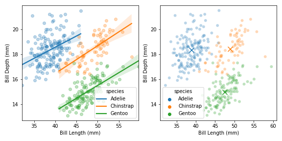
1.5. matplotlib + seaborn & seaborn + matplotlib

• matplotlib과 seaborn이 자유롭게 섞일 수 있습니다.

  • matplotlib 산점도 위에 seaborn 추세선을 얹을 수 있고,
  • seaborn 산점도 위에 matplotlib 중심점을 얹을 수 있습니다.

• 파이썬 코드는 다음과 같습니다.

  fig, axes = plt.subplots(ncols=2, figsize=(8, 4))
  
  species_u = penguins["species"].unique()
  
  # plot 0 : matplotlib + seaborn
  for i, s in enumerate(species_u):
      # matplotlib 산점도
      axes[0].scatter(penguins["bill_length_mm"].loc[penguins["species"]==s],
                     penguins["bill_depth_mm"].loc[penguins["species"]==s],
                     c=f"C{i}", label=s, alpha=0.3
                    )
                    
      # seaborn 추세선
      sns.regplot("bill_length_mm", "bill_depth_mm", data=penguins.loc[penguins["species"]==s], 
                  scatter=False, ax=axes[0])
      
  axes[0].legend(species_u, title="species")
  axes[0].set_xlabel("Bill Length (mm)")
  axes[0].set_ylabel("Bill Depth (mm)")
  
  # plot 1 : seaborn + matplotlib
  # seaborn 산점도
  sns.scatterplot("bill_length_mm", "bill_depth_mm", hue="species", data=penguins, alpha=0.3, ax=axes[1])
  axes[1].set_xlabel("Bill Length (mm)")
  axes[1].set_ylabel("Bill Depth (mm)")
  
  for i, s in enumerate(species_u):
      # matplotlib 중심점
      axes[1].scatter(penguins["bill_length_mm"].loc[penguins["species"]==s].mean(),
                     penguins["bill_depth_mm"].loc[penguins["species"]==s].mean(),
                     c=f"C{i}", alpha=1, marker="x", s=100
                    )
  
  fig.tight_layout()

  

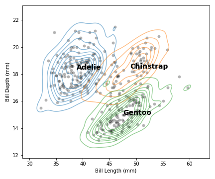
1.6. seaborn + seaborn + matplotlib

• 안 될 이유가 없습니다.
• seaborn scatterplot + seaborn kdeplot + matplotlib text입니다.

  fig, ax = plt.subplots(figsize=(6,5))
  
  # plot 0: scatter plot
  sns.scatterplot("bill_length_mm", "bill_depth_mm", color="k", data=penguins, alpha=0.3, ax=ax, legend=False)
  
  # plot 1: kde plot
  sns.kdeplot("bill_length_mm", "bill_depth_mm", hue="species", data=penguins, alpha=0.5, ax=ax, legend=False)
  
  # text:
  species_u = penguins["species"].unique()
  for i, s in enumerate(species_u):
      ax.text(penguins["bill_length_mm"].loc[penguins["species"]==s].mean(),
              penguins["bill_depth_mm"].loc[penguins["species"]==s].mean(),
              s = s, fontdict={"fontsize":14, "fontweight":"bold","color":"k"}
              )
  
  ax.set_xlabel("Bill Length (mm)")
  ax.set_ylabel("Bill Depth (mm)")
  
  fig.tight_layout()

  

1.7. 결론

• seaborn을 matplotlib과 마음껏 섞어쓰세요
• 단, axes를 반환하는 명령어에 한해서 말입니다.
• 이런 명령어를 axes-level function 이라고 합니다.