Spines & Grids

2020-08-27

2020-11-27

cognitive science, grid, matplotlib, python, spines, visualization

착시를 줄여주는 축과 격자를 설정하는 방법입니다.
matplotlib에서는 Axes.spines와 Axes.grid 객체를 통해 제어합니다.

Claus Wilke, “데이터 시각화 교과서”, 영문판(Free)
Colin Ware “데이터 시각화, 인지과학을 만나다”
White Paper-Principles of Data Visualization-What we see in a Visual

1. 착시

wikipedia: optical illusion
wikipedia: Lateral inhibition

우리 눈은 사물을 있는 그대로 보지 않습니다.
- 주변과 견주어보기도 하고, 우리가 알고 있는 지식에 비추어 보기도 합니다.
- 이런 과정에서 있는 그대로 보지 못하는 착시가 발생합니다.

착시는 생물학적 이유로 발생하기도 하는데, 예로 Mach Bands가 있습니다.
- 선이 점점 두꺼워지다 다른 선과 닿는 순간 경계 지점에 그림자가 보입니다.
- 측면 억제lateral inhibition라는 현상이 있습니다. 경계를 명확히 인지하기 위해 이렇게 진화한 것으로 생각되는데, 자극을 강하게 받은 신경 세포는 이웃한 신경세포에 억제성 신경전달 물질을 전달해서 활성화를 억제합니다.
- 그렇기 때문에 같은 색이라고 해도 다른 색과 접한 부분은 다르게 인식됩니다.
- 참고로, 이 현상을 밝힌 마하Ernst Mach는 초음속에 대한 연구를 한 그 마하입니다.

Mach Bands

한편으로 인지 방식에 의해 일어나기도 합니다.
- 우리는 배경에 비추어 물체를 인식하고 크기를 판단하기 때문입니다.
- 폰조 착시Ponzo Illusion가 대표입니다.
- 철길 그림 위의 두 막대기는 멀리 있는 것이 길어보입니다.

Ponzo Illusion

착시는 누구나 겪는 일이지만, 간단히 벗어날 수 있습니다.
- 이미 위 그림에서 선들이 닿기 전 배경선이 보일 때,
- 그리고 철길 위에 빨간 보조선을 그었을 때
- 우리는 착시에서 벗어나는 경험을 했습니다.
matplotlib에서는 spines와 grid의 도움을 받을 수 있습니다.

2. 윤곽선 `spines`

matplotlib: matplotlib.spines
matplotlib: Source code for matplotlib.spines
matplotlib: Spines
matplotlib: Dropped spines
matplotlib: Spine Placement Demo
matplotlib: Centered spines with arrows

matplotlib에서 부르는 이름은 조금 낯설지만 생각해보면 은근 직관적입니다.
- 제가 축공간이라고 부르는, 그림이 그려지는 공간은 axes이고
- 눈금이 붙는 부분의 이름은 spines입니다.
데이터 시각화 교과서에는 spine에 대한 언급이 별로 없습니다.
- 보여주고자 하는 데이터의 종류에 따라 다르고
- 특히 그림의 종류에 따라 적절히 변형되어 사용되고 있습니다.
- 원하는 형식으로 연출할 수 있도록 이번 글은 기능 위주로 작성하겠습니다.

데이터 시각화 교과서에 수록된 그림들

matplotlib의 object oriented interface에서, spine은 ax.spines로 제어됩니다.

지난 글에 있는 코드를 그대로 활용하고, ax.spines 활용에 집중하기 위해 시각화 코드를 함수로 만들어 버립니다.

def plot_example(ax, zorder=0):
    ax.bar(tips_day["day"], tips_day["tip"], color="lightgray", zorder=zorder)
    ax.set_title("tip (mean)", fontsize=16, pad=12)

    # Values
    h_pad = 0.1
    for i in range(4):
        fontweight = "normal"
        color = "k"
        if i == 3:
            fontweight = "bold"
            color = "darkred"

        ax.text(i, tips_day["tip"].loc[i] + h_pad, f"{tips_day['tip'].loc[i]:0.2f}", 
                horizontalalignment='center', fontsize=12, fontweight=fontweight, color=color)

    # Sunday
    ax.patches[3].set_facecolor("darkred")
    ax.patches[3].set_edgecolor("black")

    # set_range
    ax.set_ylim(0, 4)
    return ax

object oriented 방식은 이런 식의 호출이 가능합니다.
1
2
fig, ax = plt.subplots()
ax = plot_example(ax)

spines의 정체를 확인해봅시다.
1
type(ax.spines)

OrderedDict객체입니다. dictionary의 일종이네요.

그럼 key와 value는 어떤 것들일까요?

1 2	for k, v in ax.spines.items(): print(f"spines[{k}] = {v}")

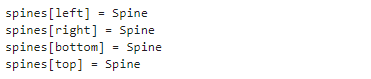
key는 "left", "right", "bottom", "top"이네요. 네 개의 테두리입니다.
value가 뭔지 잘 모르겠습니다. 다시 정체를 파악해봅니다.
1
ax.spines.values()

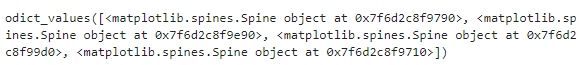
matplotlib.spines.Spine 객체입니다.
- 공식문서에 따르면 Spine은 Patch의 subclass이고
- set_patch_circle, set_patch_arc가 호출되면 원이나 호를 그리기도 한답니다.
- 선을 그리는 set_patch_line이 기본값입니다.

2.1. spine 숨기기 : `.set_visible(False)`

matplotlib.axes

위 그림에서 맨 아래만 남기고 왼쪽, 위쪽, 오른쪽 spines를 지워보겠습니다.

set_visible(False) 명령을 사용하면 됩니다.

fig, ax = plt.subplots()
ax = plot_example(ax)

ax.spines["top"].set_visible(False)
ax.spines["left"].set_visible(False)
ax.spines["right"].set_visible(False)

사족을 하나 붙이면, set_visible()은 spine에만 적용되는 명령이 아닙니다.
- General Artist Properties라고 해서 모든 객체에 적용 가능한 명령입니다.
- 위 예시에선 spine에 사용했을 뿐입니다.
- 이전 글에서 설명했듯 bar 객체에도 적용 가능합니다.

2.2. spine 범위 지정하기 : `.set_bounds(min, max)`

spine을 일부 영역만 보여주고 싶을 수 있습니다.
왼쪽 spine을 안보이게 하는 대신 가운데만 그려봅시다.

set_bounds(min, max)를 사용합니다.

fig, ax = plt.subplots()
ax = plot_example(ax)

ax.spines["top"].set_visible(False)
ax.spines["right"].set_visible(False)

ax.spines["left"].set_bounds(1, 3)

2.3. spine 위치 지정하기 : `.set_position((direction, distance))`

matplotlib.spines
matplotlib.axes.Axes.set_position
matplotlib: Spine placement demo
matplotlib: Centered spines with arrows

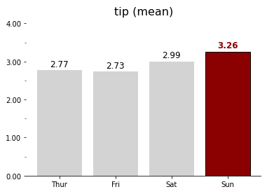
지난번 글에서 이런 그림을 그렸습니다.
가로와 세로축을 원래 위치에서 밖으로 살짝 밀어서 공간을 확보하고 여유를 연출했습니다.

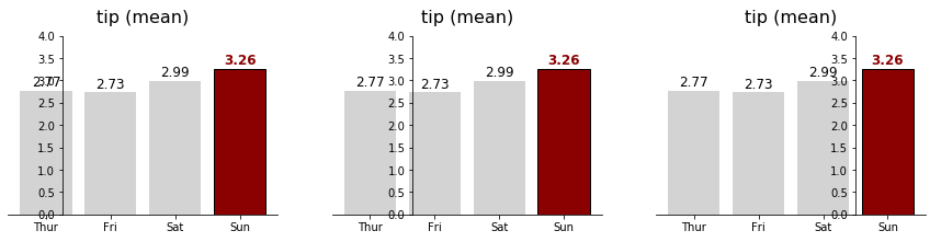
set_position((direction, distance))을 사용해서 할 수 있습니다.
먼저, get_position()을 사용해서 spines["left"]가 어떻게 설정돼있나 보겠습니다.
1
ax.spines["left"].get_position()

밖으로(“outward”) 0만큼 나가있다고 합니다.

set_position(("outward", 10))을 설정해서 조금 간격을 띄워보겠습니다.

fig, ax = plt.subplots()
ax = plot_example(ax)

ax.spines["top"].set_visible(False)
ax.spines["right"].set_visible(False)
ax.spines["left"].set_position(("outward", 10))

“outward”를 넣을 수 있으니 거꾸로 할 때는 “inward”를 쓰면 될 것 같습니다.
그렇지 않습니다. 대신 거리를 음수로 넣으면 됩니다.

“outward” 대신 “axes”, “data”를 넣을 수 있고, 의미는 다음과 같습니다.

fig, ax = plt.subplots(ncols=3, figsize=(15, 3))

for i in range(3): # 그래프 세개 한번에 그리기
    ax[i] = plot_example(ax[i])
    ax[i].spines["top"].set_visible(False)
    ax[i].spines["right"].set_visible(False)
    
# ax[0] : spine을 data 영역에서 지정된 거리만큼 이동  
ax[0].spines["left"].set_position(("outward", -50))

# ax[1] : spine을 axes의 지정된 위치에 설정
ax[1].spines["left"].set_position(("axes", 0.3))

# ax[2] : spine을 data의 지정된 위치에 설정
ax[2].spines["left"].set_position(("data", 2.5))

“axes”와 “data”도 음수를 함께 사용할 수 있습니다.

이 기능을 이용하면 수학시간에 많이 보던 형태의 그래프를 그릴 수 있습니다.

## data
x = np.linspace(-np.pi, np.pi, 100)
y = 2 * np.sin(x)

fig, ax = plt.subplots(ncols=3, figsize=(12,4))

## normal plot
ax[0].plot(x, y)
ax[0].set_title("normal plot", pad=12)

## textbook (1)
ax[1].plot(x, y)
ax[1].set_title("textbook (1)", pad=12)
# top, right 는 안보이게
ax[1].spines["top"].set_visible(False)
ax[1].spines["right"].set_visible(False)
# left, bottom은 (0, 0)을 지나가게
ax[1].spines["left"].set_position(("data", 0))
ax[1].spines["bottom"].set_position(("data", 0))

## textbook (2)
ax[2].plot(x, y)
ax[2].set_title("textbook (2)", pad=12)
# top, right 는 안보이게
ax[2].spines["top"].set_visible(False)
ax[2].spines["right"].set_visible(False)
# left, bottom은 (0, 0)을 지나가게
ax[2].spines["left"].set_position(("data", 0))
ax[2].spines["bottom"].set_position(("data", 0))
# 화살표 추가
ax[2].plot(1, 0, ">k", transform=ax[2].get_yaxis_transform(), clip_on=False)
ax[2].plot(0, 1, "^k", transform=ax[2].get_xaxis_transform(), clip_on=False)

plt.show()

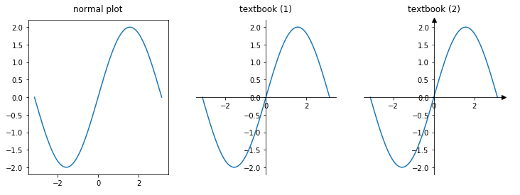
자주 사용할 것들은 이렇게 간단히 사용할 수 있습니다.
- set_position(("axes", 0.5")) 대신 set_position("center")
- set_position(("data", 0.0")) 대신 set_position("zero")

3. 격자`grid`

matplotlib.axes.Axes.grid

spines를 적절히 잡아주면 데이터를 읽기 좋아집니다.
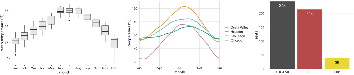
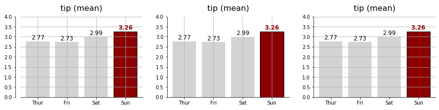
그러나 데이터간 크기를 더 잘 비교하려면, 그림에 grid를 깔아주면 더 좋습니다.

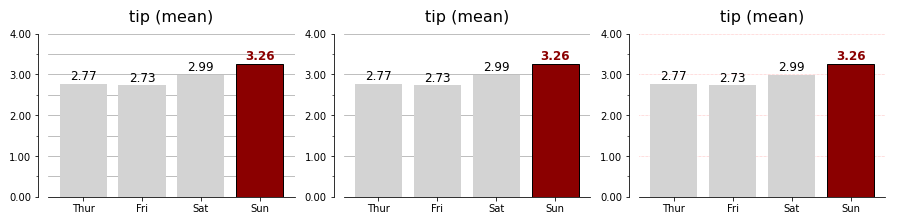
.grid(True) 메소드로 격자를 그릴 수 있습니다.

axis={“both”, “x”, “y”} 인자로 방향을 지정합니다.

fig, ax = plt.subplots(ncols=3, figsize=(15, 3))

for i in range(3): # 그래프 세개 한번에 그리기
    ax[i] = plot_example(ax[i])
    ax[i].spines["top"].set_visible(False)
    ax[i].spines["right"].set_visible(False)
    ax[0].spines["left"].set_position(("outward", 10))
    
# ax[0] : x, y 둘 다 
ax[0].grid(axis="both")

# ax[1] : x축에서만
ax[1].grid(axis="x")

# ax[2] : y축에서만
ax[2].grid(axis="y")

3.1. major and minor ticks

matplotlib: major and minor ticks

grid는 major와 minor tick을 구분하여 그릴 수 있습니다.

먼저, major와 minor tick을 설정합니다.

from matplotlib.ticker import (MultipleLocator, AutoMinorLocator)

fig, ax = plt.subplots()
ax = plot_example(ax)

# top, right, left spines 안보이기
ax.spines["top"].set_visible(False)
ax.spines["right"].set_visible(False)
ax.spines["left"].set_visible(False)

# y축 tick 설정
ax.yaxis.set_major_locator(MultipleLocator(1))    # major tick을 1 단위로 설정
ax.yaxis.set_major_formatter('{x:0.2f}')          # major tick format 지정 (오류가 나면 matplotlib upgrade)
ax.yaxis.set_minor_locator(MultipleLocator(0.5))  # minor tick을 0.5 단위로 지정

plt.plot()

3.2. major grid only

major와 minor ticks가 구분되면, 한쪽을 선택해서 그릴 수 있습니다.
major와 minor grid를 구분해서 지정할 수 있습니다.

따라서, 색상이나 선 스타일 등을 구분해서 변화시키기 좋습니다.

fig, ax = plt.subplots(ncols=3, figsize=(15, 3))

for i in range(3): # 그래프 세개 한번에 그리기
    ax[i] = plot_example(ax[i], zorder=2) # zorder: bar를 grid 앞으로.
    ax[i].spines["top"].set_visible(False)
    ax[i].spines["right"].set_visible(False)
    ax[i].spines["left"].set_position(("outward", 10))
    ax[i].yaxis.set_major_locator(MultipleLocator(1))
    ax[i].yaxis.set_major_formatter('{x:0.2f}')
    ax[i].yaxis.set_minor_locator(MultipleLocator(0.5))
    
# ax[0] : major, minor 둘 다
ax[0].grid(axis="y", which="both")

# ax[1] : major만
ax[1].grid(axis="y", which="major")

# ax[2] : major만 + 여러 옵션
ax[2].grid(axis="y", which="major", color="r", ls=":", lw=0.5, alpha=0.5)

plt.show()

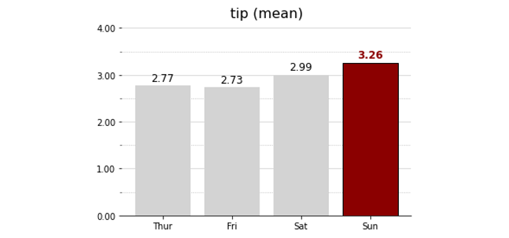
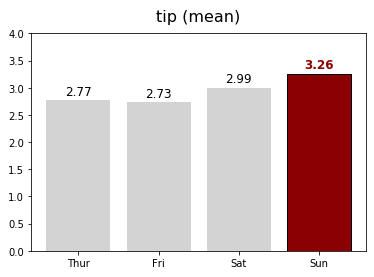
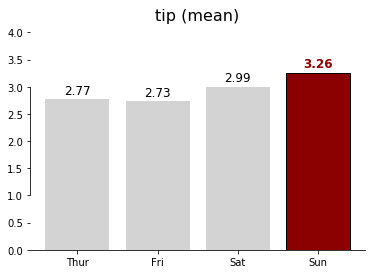
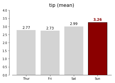
최종적으로 다음과 같은 결과물을 얻을 수 있습니다.
불필요한 spine을 제거해서 시선 분산을 막고,

grid를 추가해서 데이터들을 옆에 있는 숫자들과 비교하기 좋게 했습니다.

fig, ax = plt.subplots()
ax = plot_example(ax, zorder=2)

ax.spines["top"].set_visible(False)
ax.spines["right"].set_visible(False)
ax.spines["left"].set_visible(False)
    
ax.yaxis.set_major_locator(MultipleLocator(1))
ax.yaxis.set_major_formatter('{x:0.2f}')
ax.yaxis.set_minor_locator(MultipleLocator(0.5))

ax.grid(axis="y", which="major", color="lightgray")
ax.grid(axis="y", which="minor", ls=":")

도움이 되셨나요? 카페인을 투입하시면 다음 포스팅으로 변환됩니다

PythonData Science

1. 착시

2. 윤곽선 spines

2.1. spine 숨기기 : .set_visible(False)

2.2. spine 범위 지정하기 : .set_bounds(min, max)

2.3. spine 위치 지정하기 : .set_position((direction, distance))

3. 격자grid